Spectrum-Slicing

*Disclaimer* - This library and the accompanying documentation are still in development. If you find any bugs, have any suggestions, or find any documentation that is confusing, please post an issue. It will help make this library better for future users.

The Shift-and-Invert Parallel Eigenproblem Solver (SIPS) also known as the Spectrum-Slicing algorithm is a numerical method for solving large eigenvalue problems or generalized eigenvalue problems . The crux of the algorithm is to divide the eigenspectrum into slices which can be solved independently. Because each slice can be solved independently, interprocess communication is kept to a minimum, and efficient performance is maintained up to very large matrices with a very large number of processes in use. An implementation of the spectrum-slicing algorithm demonstrated good performance up to a N=500,000 matrix with n=200,000 processes.[Ref] Like many high-performance algorithms, Spectrum-Slicing features numerous controls, optimization strategies, and difficulties that may arise based on the specifics of the problem. Although the algorithm has typically been applied to large-scale problems, it is the opinion of the author that the characteristics of the algorithm also make it an excellent choice for many small and medium-sized problems. Therefore, this library provides general use interfaces to facilitate easy addition of computer power to your existing code. The library is built on top of PETSc and SLEPc; at least version 3.9 of each is required and tests were performed on PETSc 3.9.3 and SLEPc 3.9.2

Goals of this library:

1. Provide easy-to-use interfaces which work well in most situations. Currently, 3 interfaces are provided of gradually increasing difficulty of use (dsygvs, dsygvsx, and SIPSsolve).
2. Explain the basic performance considerations of the algorithm, limitations, effective strategies, and available controls.

Table of Contents:

• Is the Spectrum-Slicing algorithm the right solution to my problem?
• How do I use the Spectrum-Slicing algorithm?
• dsygvs - Solving a square matrix
• dsygvsx - Expert Driver for square matrices
• SIPSolve - Solver for PETSc matrices
• Performance characteristics and theory
• Load Balancing
• Time to solution versus sparsity
• Time to solution versus number of processors
• Suggested route to solution for different problem sizes

Is the Spectrum-Slicing algorithm the right solution to my problem?

The spectrum slicing algorithm may be appropriate for your problem if all the following conditions are met:

1. The matrix to be diagonalized is sparse and symmetric
2. The matrix is real (At present only routines for real matrices are presented. Routines for complex matrices will be available in a future release, however they will be restricted to full multicommunicator mode which will limit problem size).

Additionally at least one of the following must be true for reasonable performance:

1. The eigenspectrum is nearly linearly distributed.
2. A rough idea of the probability distribution of the eigenspectrum is known a priori.
3. The eigenspectrum will be solved repeatedly.
4. The problem will be solved with few processes.

Optionally, the algorithm can make use of a speedup from computing only a portion of the eigenspectrum.

How do I use the Spectrum-Slicing algorithm?

Compiling the code

First the user must install PETSc and SLEPc at least versions 3.9. The only configure option recommended of PETSc is to use --with-debugging=0. (Future versions of this library which will implement the multiple processes per slice architecture for large problems may require MUMPS, ParMetis, and PT-Scotch) Next, the user must ensure that the environmental variables PETSC_DIR, SLEPC_DIR, and PETSC_ARCH are set according to their PETSc/SLEPc installation. Also, the user must set the variables SIPS_DIR, LD_LIBRARY_PATH (to contain SIPS_DIR), OMP_NUM_THREADS=1, and (optionally) SCALAPACK_DIR. The file setenv contains prototypes of these definitions and can be loaded with the source command in bash.

To compile change to the SIPS directory and call

make

This will compile libsips.so, libsips_square.so, and sips_square. The code can be tested by calling

make test

Additional information about the test program sips_square can be found by running sips_square -h, or by examining the examples in the makefile.

Using the code

In order to use the code, the header files which describe the available functions should be included:

#include <sips.h>

or

#include <sips_square.h>

Likewise, fortran users can import interfaces to the libraries in sips.F90 and sips_square.F90.

The libraries containing the compiled code should be linked by the compiler by adding -L${SIPS_DIR} and by using -lsips and/or -lsips_square.

Finally, the code should be changed to call the sips eigensolver.

Assuming your code uses a serial eigensolver (e.g. dsyev from Lapack), then the sips_square eigensolver can be utilized by replacing the call to the serial eigensolver with either the simple (dsygvs) or complex sips_square (dsygvsx) driver, and when running the program call it with

mpiexec -n n_procs my_program

The program will run through serial execution where each process performs the same calculation in order to set up the matrix (presumably there will be a global computational cost of O() to set up the matrix). Then each process will call the eigensolver, where the process will be assigned a slice and solve its slice (global computational cost O()). The sips_square routines are set up to gather the solution so that every process ends up with the entire set of eigenvalues and eigenvectors. When the processes leave the call to the solver, they resume their serial execution with each process performing the same operations on its local copy of the matrix. If other O() computations are necessary, then additional parallelism is needed (e.g. the SIPSolve driver).

dsygvs - Solving a square matrix

The definition of dsygvs is:

int dsygvs(int 	*N, double  *A, double  *B, double 	*W)

N is the size of the matrix. A and B are square NxN matrices. On output A contains the eigenvectors and W (an array of size N) contains the eigenvalues. If an eigenvalue problem but not a generalized eigenvalue problem is desired, then NULL can be passed instead of matrix B. dsygvs makes many default assumptions and is equivalent to calling dsygvsx with NULL for all values besides N,A,B, and W.

dsygvsx - Expert Driver for square matrices

The definition of dsygvsx is:

int dsygvsx( int *N, double *A, double *B, double *W, PetscInt interval_optimization, double *interval, int prev_eigenvalues, char *JOBZ, char *UPLO)

NULL is accepted to set the default behavior for B, interval_optimization, interval, prev_eigenvalues, JOBZ, and UPLO.

If previous eigenvalues are provided, by specifying the number of eigenvalues in the argument prev_eigenvalues, and those eigenvalues are placed in W, then the previous eigenvalues will be used to create a eigenvalue distribution and the driver will create slices with roughly the same of eigenvalues in each slice. Additionally, W does not have to contain actual eigenvalues and could instead be used to specify an expected probability distribution. For instance, if the values places in W are logarithmically distributed, then the slices created will be logarithmically distributed. The the values used to set the subintervals do not span the entire eigenspectrum, then on exit, N will contain the number of eigenvalues/eigenvectors found.

If the previous eigenvalue option has not been set, the driver will next turn to the interval and interval_optimization options. If interval optimization is turned on (default), then the driver will use matrix inertia calculations to enlarge and then shrink the interval so that the entire eigenspectrum is contained in the interval. The slices will then be uniformly distributed throughout the interval. If interval optimization is turned off, then it will be assumed that interval[0] is the left end of the interval to be solved and interval[1] is the right end. On exit, N will contain the number of eigenvalues/eigenvectors found.

Like Lapack, the JOBZ argument can be used to control whether the eigenvectors overwrite A on exit and the eigenvalues overwrite W on exit (using the value 'V' or 'V' (default)) or only the eigenvalues overwrite W on exit (using the value 'N' or 'n')

Like Lapack, UPLO can be used to specify that only the upper or lower triangle of the matrix has been provided. UPLO='U' or 'u' for upper and UPLO='L' or 'l' for lower. The missing triangle will be filled in by symmetry before solving. The default option is neither and the passed matrices are assumed to be symmetric.

SIPSolve - Solver for PETSc matrices

The definition of SIPSolve is:

PetscErrorCode  SIPSolve(Mat *A_pttr, Mat *B_pttr, PetscReal *interval, PetscInt interval_optimization, PetscReal *eig_prev, PetscInt nEigPrev, EPS  *returnedeps)

A_pttr - pointer to PETSc matrix A. It was chosen to make this a pointer to facilitate communication with fortran. B_pttr - pointer to PETSc matrix B.

interval, interval_optimization, eig_prev, and nEigPrev behave the same as in dsygvx including with regards to passing of NULL to enable default options.

returnedeps returns the Eigen Problem Solver object from the SLEPc library. The EPS object contains the solution (eigenvalues and eigenvectors) to the problem. These can be obtained by a call to eigenvaluesFromEPS(EPS *epsaddr,double *W,int N), int eigenvectorsFromEPS(EPS *epsaddr,PetscScalar *A,int N), or simultaneous with squareFromEPS(EPS *epsaddr,PetscScalar *A,double *W,int N). A lot of memory is used by the EPS object and should be cleaned up by EPSDestroy.

What are the important knobs and performance characteristics of the solver?

Load Balancing

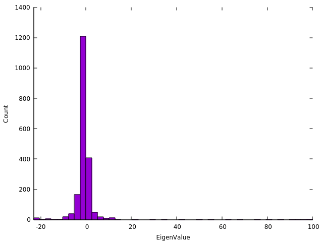
The time taken for a slice to be solved is proportional to the number of eigenvalues in the slice, although this is not the only consideration. From this assumption, it follows that the time to completion is proportional to the maximum number of eigenvalues in any slice. A good first guess to achieving proper load balancing, is to aim for each subinterval to contain an equal number of eigenvalues. Here is the spectrum of a matrix which results in poor load balancing using the defaul options. This matrx was created using:

./sips_square -rows 2000 -nonzerodiagonals 100

The eigenvalues have been binned into 48 bins as this matrix was diagonalized and timed with 1-48 processes. It is apparent that a single slice contains more than half the eigenvalues.

Time to solution versus sparsity

Many users wish to know what algorithm will solve their problem the fastest. If you estimate the time to solution for each algorithm on a single process, and know the soft scaling behavior of the algorithm as the number of processes is increased, then an estimate of which algorithm will be faster is straightforward.

Therefore, here we compare the time to solution of the spectrum slicing algorithm (dsygvs) and lapack (dsygv) versus the problem size (N, set using the -rows option of sips_squaretest) and the sparsity (controlled using the -nonzerodiagonals option of sips_squaretest). The matrices produced were diagonalized by both algorithms and were timed using the time command.

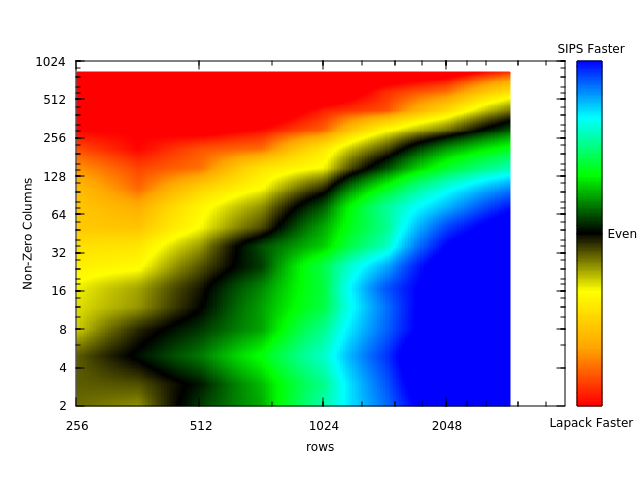
Each color shade represents a factor of 2 difference in speed. We find roughly equal speed between the lapack and sips calls when 1/16th (about 6%) of the matrix is nonzero.

Because the spectrum slicing algorithm maintains nearly the same process efficiency (assuming proper load balancing) as the number of processes increases, if SIPS is faster for a single process it will also likely be faster for parallel runs. Additionally, some of the area of the graph which shows lapack being faster, may shift to SIPS being faster when parallelism is considered based on the parallel performance of the other algorithm.

Time to solution versus number of processors

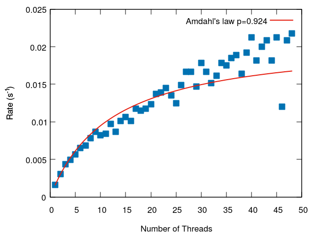
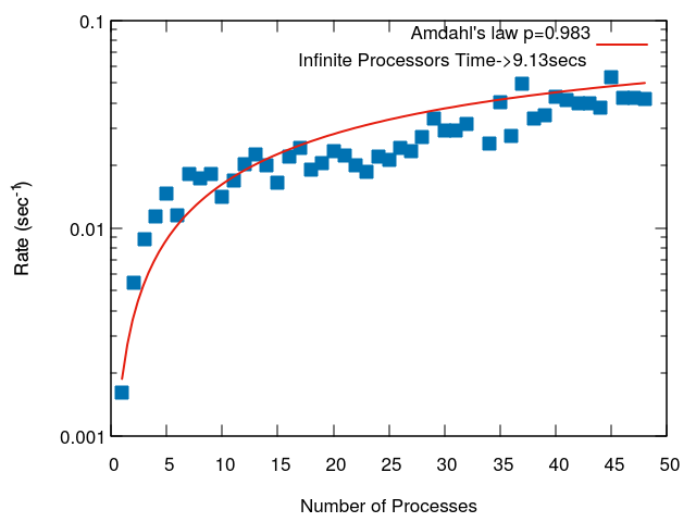
Here we present two diagonlization tests which measure the time to solution versus the number of processes. The two tests different in the way load-balancing was achieved. In each case we fit the run time to Amdahl's law. Amdahl's law assumes the run time can be divided into parallel and serial components. Although the actual run time versus the number of processors for spectrum-slicing does not match the shape of the Amdahl's law curve (the run time is all parallel, but affected by load balancing), it is still a useful means to compare the parallel performance, and the "serial" portion is in some ways similar to the process which was given the largest load.

Matrix with nearly uniform distribution of eigenvalues

The first test is of a matrix with an eigenspectrum that is distributed like a cosine function. The matrix had 4000 rows and 184 nonzero entries in each row. The speed to achieve diagonalization was timed with 1-48 processes. 1 process took 619 seconds, and 48 processes took 46 seconds (13.5x speedup).

Repeated solving of matrices with similar eigenvalue distributions

This next test is of a matrix with a very poor eigenspectrum distribution. The first diagonalization used uniformly distributed subintervals. The second diagonalization used the eigenvalues from the previous run to distribute the subintervals. This test was ran using the -doublediag option of sips_square. It can be seen that the first diagonalization only achieved a speed up of about 4x using 48 processors aside from a few points which had a better balance.

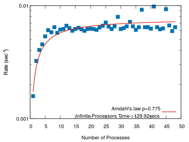
We are trying to encode a strategy that will address this slow first run problem by sampling the inertia before the first diagonlization, however, inertia calculations can be costly and we do not yet have a proper cost-benefit analysis for this strategy.

The second run which used the output of the first run to seed the second run resulted in a speedup of 26x on 48 processes.

Route to Solution Versus Problem Size

Regardless of what size your problem is, load balancing is a major issue. Be sure to understand the basic difficulties of load balancing in the spectrum-slicing algorithm.

The dense matrix fits within the memory available to a single process.

The smallest problem size worth mentioning. Here the recommended solution is to use the sips_square drivers. These are by the far the simplest to use and will require minimal changes to your code. Although there are some superfluous calls, they have a computational cost of O() and are not significant compared to the diagonalization cost of O(). The per-process memory usage will be times 8 (double precision) or 16 (complex double precision) times a small multiplier (1-5). The performance increases efficiently with the number of processes in this region, but because of the limited system size calculations can become fast enough with ~100 processes that there is almost no utility in adding more.

The sparse matrix fits within the memory available to a single process.

Here you will have to use the more complex driver SIPSolve. This will require assembling PETSc matrices directly without allocating dense matrices. If n<<N, then aseembling PETSc matrices and other O() operations can still be carried out in series and this will not significantly affect performance. The diagonalization should be done in full multicommunicator mode (i.e. 1 process/slice. currently, this is the only option, but in the future it will be the default option). This will result in each process having a full copy of the sparse matrix during solving which uses more memory than other solvers, but it comes with greater speed. The performance remains quite efficient throughout this entire range.

The sparse matrix cannot fit within the memory available to a single process

This will require setting more than 1 process/slice (not currently implemented, see EPSKrylovSchurSetIntervals). As the number of processes per slice goes up, the efficiency will go down drastically. However, this is necessary to fit the matrix in memory. This is not currently implemented, and you will have to deviate from the code of SIPSolve to implement this. It is recommend to keep the number of processes per slice to a minimum to achieve diagonalization in the least time, but it should be sufficient to provide enough memory for the matrix. NOTE At present there is little we can do to make this available for complex matrices. The mumps package which will be used to allow more than 1 process/slice for real matrices does not provide an inertia calculation for complex matrices. Therefore, complex eigenvalue problems in this size range will likely remain unsolvable by SIPS for the near future.

Description of contents

sips.c / libsips.so

SIPSShowInertias(EPS eps) -prints the subintervals and inertias

SIPSShowVersions() -prints the version of PETSc and SLEPc used

SIPSShowErrors(EPS eps) -prints errors resulting from EPSSolve

SIPSIntervalOptimization(EPS eps,double *interval) performs the interval optimization starting with the left end, interval[0], and the right end, interval[1]. On exit, and optimized interval is returned and set to the EPS object.

SIPSolve(Mat *A_pttr, Mat *B_pttr, PetscReal *interval, PetscInt interval_optimization, PetscReal *eig_prev, PetscInt nEigPrev, EPS *returnedeps) Given matrix A, and [optionally] matrix B, along with the other options, this performs a diagonlization using the spectrum slicing object. On output the solution is stored in returnedeps.

SIPSCreateDensityMat(EPS *epsaddr, double *weights, int N, Mat *P) This takes an EPS object along with a set of weights for each eigenvector and returns a PETSc matrix, P, which is a density matrix.

sipssquare.c / libsips_square.so

LTtoSym(PetscScalar *matrix, int rows, int columns)

UTtoSym(PetscScalar *matrix, int rows, int columns)

dsyevs(int *N, double *A, double *W)

dsygvs(int *N, double *A, double *B, double *W)

dsygvsx( int *N, double *A, double *B, double *W, PetscInt interval_optimization, double *interval, int prev_eigenvalues, char *JOBZ, char *UPLO)

eigenvaluesFromEPS(EPS *epsaddr,double *W,int N)

eigenvectorsFromEPS(EPS *epsaddr,PetscScalar *A,int N)

double listmax(double *list, int num)

double listmin(double *list, int num)

void printdatatypes()

printmatrix(double *matrix, int rows, int cols, int stride, int rowmajor, int brief)

squareFromEPS(EPS *epsaddr,PetscScalar *A,double *W,int N)

Mat squareToPetsc(PetscScalar *A, int N)

sips_squaretest.c / sips_square executable