Project 4 — Advanced Lane Line Finding, part of Udacity’s Self-Driving Car Nanodegree Program (www.udacity.com)
(See this post on Medium: https://medium.com/@arnaldogunzi/advanced-lane-line-project-7635ddca1960)
In this project, the challenge is to create a improved lane finding algorithm, using computer vision techniques. The result must be something like this:

And here is a video illustrating the final result of the technique.
https://youtu.be/gRFs_PjR_LU
This is the fourth project of the nanodegree. The second one heavily focused on computer vision, mainly using the opensource package OpenCV (Open Computer Vision). The two other projects used machine learning, with deep neural networks. This project has following steps
1 Camera calibration
2 Color and gradient threshold
3 Birds eye view
4 Lane detection and fit
5 Curvature of lanes and vehicle position with respect to center
6 Warp back and display information
7 Sanity check
8 Video
Each of them will be briefly exposed here.
The first step of the project is to do the camera calibration. It is necessary because the lenses of the camera distort the image of the real world. The calibration corrects this distortion. It works like glasses correcting an myopic eye.
The first question: what is the degree of “myopia”? To find this, we do a lot of tests in the ophthalmologist.
In our case, we also do a lot of tests. But with chessboards. Chessboards are great, because it is a regular pattern of squares. We know how is the original pattern and how the camera is showing it. Having at least 20 images of chessboards in different angles, we can use opencv function cv2.calibrateCamera() to find the arrays that describe the distortion of the lenses. Then, we can apply cv2.undistort() function.

Here are an example using test images.

Note the difference in the corners of images
Input: Images from cameras
Output: Undistorted images
We want to detect the lanes of the road. Not the trees. Not other cars (not yet, we will do this in the next project).
We use color and gradient thresholds to filter out what we don’t want. We know some features of the lanes: they are white or yellow. There is a high contrast between road and lanes. And they form an angle: they are not totally vertical or horizontal in image.
We do a color threshold filter to pick only yellow and white elements, using opencv convert color to HSV space (Hue, Saturation and Value). The HSV dimension is suitable to do this, because it isolates color (hue), amount of color (saturation) and brightness (value). We define the range of yellow independent on the brightness (for example, in shadow or under the sun). At least in theory. In practice, the tuning of “yellowness” is a matter of trial-and-error. I based the values on the diagram below and in the post of Vivek Yadav (https://medium.com/towards-data-science/robust-lane-finding-using-advanced-computer-vision-techniques-mid-project-update-540387e95ed3#.hfm1xx73q).


yellow_low = np.array([0,100,100]) yellow_high = np.array([50,255,255])
white_low = np.array([18,0,180]) white_high = np.array([255,80,255])
To find the contrast, we use the Sobel operator. It is an derivative, under the hood. If the difference in color between two points is very high, the derivative will be high.
But we can compare any two neighbor points to do this derivative. The images below show a filter in an arbitrary direction threshold and only on x direction.
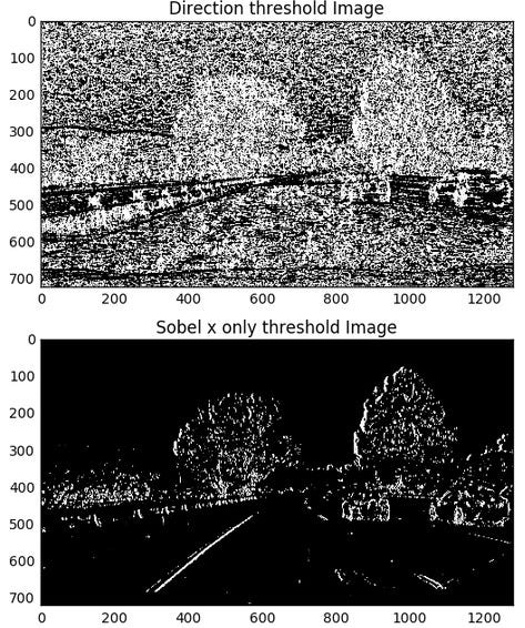
By tuning the threshold parameters, we can have an estimate of the lanes. In the end, I used only the x direction threshold, because some other directional thresholds included a lot of noise.
Finally, I did a bitwise addition of the three masks: yellow, white and sobelX thresholds.
Input: undistorted image Output: binary image with lanes
The idea here is to warp the image, as if it is seem from above. That is because makes more sense to fit a curve on the lane from this point of view, then unwarp to return to the original view.
Here we are considering the camera is mounted in a fixed position, and the relative position of the lanes are always the same.
The opencv function warp needs 4 origins and destinations points. The origins are like a trapezium containing the lane. The destination is a rectangle.
Source — Destination 585, 460–320, 0 203, 720–320, 720 1127, 720–960, 720 695, 460–960, 0
The effect of this transformation is.

Another example

Input: binary image with lanes Output: birds eye view
We are using second order polynomial to fit the lane: x = ay**2 + by + c.
In order to better estimate where the lane is, we use a histogram on the bottom half of image.

The idea is that the lane has most probability to be where there are more vertical points. Doing this, we find the initial point.
Then we divide the image in windows, and for each left and right window we find the mean of it, re-centering the window.
The points inside the windows are stored.
We then feed the numpy polyfit function to find the best second order polynomial to represent the lanes, as in image below.


Input: birds eye view Output: curves of the lanes
In a given curve, the radius of curvature in some point is the radius of the circle that “kisses” it, or osculate it — same tangent and curvature at this point.
This link has a great tutorial on it. http://www.intmath.com/applications-differentiation/8-radius-curvature.php

It is important to know this because it will be a indicative to the steering angle of the vehicle.
The radius of curvature is given by following formula.
Radius of curvature= (1 + (dy/dx)**2)**1.5 / abs(d2y /dx2)
We will calculate the radius for both lines, left and right, and the chosen point is the base of vehicle, the bottom of image.
x = ay2 + by + c
Taking derivatives, the formula is: radius = (1 + (2a y_eval+b)**2)**1.5 / abs(2a)
in the point where x = 0, represented as y_eval in the formula. Another confusion point is that x = 0 if the orientation is upside down, but the coordinates of image is downside -up. Then x = bottom of image, in the case, 720 pixels.
Another consideration. The image is in pixels, the real world is in meters. We have to estimate the real world dimension from the photo.
I’m using the estimative provide by class instructions:
ym_per_pix = 30/720 # meters per pixel in y dimension xm_per_pix = 3.7/700 # meters per pixel in x dimension
Applying correction and formula, I get the curvature for each line.
Example values: 632.1 m 626.2 m
The offset to the center of lane.
We assume the camera is mounted exactly in the center of the car. Thus, the difference between the center of the image (1280 /2 = 640) and the middle point of beginning of lines if the offset (in pixels). This value times conversion factor is the estimate of offset.
((xL(720) + xR(720))/2–1280/2 )* xm_per_pix
Input: curves of the lanes Output: radius of curvature and offset from center
Once we know the position of lanes in birds-eye view, we use opencv function polyfill to draw a area in the image. Then, we warp back to original perspective, and merge it to the color image.
We can compose the output image with some other images, to form a diagnostic panel. It is easy done, remembering that an image is just an numpy array. We can resize it, and position this resized image in the output image.
a) Composition of images to final display img_out=np.zeros((576,1280,3), dtype=np.uint8)
img_out[0:576,0:1024,:] =cv2.resize(img_merge,(1024,576))
b) Threshold
img_out[0:288,1024:1280, 0] =cv2.resize(img_mag_thr*255,(256,288))
img_out[0:288,1024:1280, 1] =cv2.resize(img_mag_thr*255,(256,288))
img_out[0:288,1024:1280, 2] =cv2.resize(img_mag_thr*255,(256,288))
c)Birds eye view img_out[310:576,1024:1280,:] =cv2.resize(img_birds,(256,266))
One trick here. The threshold image has just one channel. So I fed it three ones, one for each color channel.
Input: curves of the lanes, radius of curvature and offset from center Output: image with lanes drawn on it
-
I tried to calculate the difference between lines in 2 points. Did not work, because the width of project video and challenge video is different. So, this method should be tuned for every new lane. Therefore, it is not robust.
-
Lines more of less parallel: so derivative in two points have to be about the same. I used this difference of derivatives as a sanity check.
If the lane fit don’t pass the sanity check, we use the last good fit.
Everything here was done in single images. How about a video? A video is a lot of images, in sequence. Python has the good package moviepy, to make easy to work with videos. For each frame of the video, we apply all techniques shown, and feed back the treated image in video.
Because a video has a lot of images in sequence, in some of these images the algorithm can not work well. In these cases, we can use the last good historic images to help. Of course, we can not use future images, it would be a non-causal model, useless for real-time applications.
Project video: good performance of this model.
Challenge video: it didn’t perform so that well.
A useful tip from my mentors. To process only the portion of video with problems, you can find a subclip of it
clip1 = VideoFileClip("project_video.mp4").subclip(22,26) #From 22s to 26 s
The technique shown works very well to the situation it was design for. For example, it picks the yellow and white lanes, so it will not work well in situations were panes are blue, or pink, for example. Or when the curves are outside the chosen boundary region (and a too broad region will introduce noise). The overtuning of parameters will make it not able to generalize the method.
Computer vision techniques are straigthforward, in comparison to recognition by deep learning for example. By straightforward, I mean we explicitly define the steps we want to take (undistort, detect edges, pick colors, and so on). By the other hand, in deep learning we do not explicitly choose these steps. Deep learning can make the algorithm more robust sometimes, other times make it fail for reasons nobody knows why.
Perhaps the best conclusion to take is that it is easy to create a simple algorithm that performs relatively well, but it is very very hard to create one that will have a human level performance, to handle every situation. There are a lot of improvements to be done. Imagine a lane finding algorithm at night? Or under rain? Perhaps a combination of approachs can make the final result more robust. Or the algorithm can have different tunings for different roads, for example.
In Brazil, it is a common situation to do not have road lanes at all!
I would like to thanks Udacity for providing this high level challenge.
I wanted to see how is the vision of HLS and HSV channels, in order to pick the parameters to tune the filters.
HLS view:

Note S and L channels are better to find lanes
HSV view:

S and V channels are better to find lanes