Benchmark Dose Analysis

Introduction

Benchmark dose analysis consists of fitting dose-response data to a collection of parameterized equations (models), followed by averaging over those models to find the BMD, or choosing the model that best describes the data while minimizing complexity (i.e., the best fit model). Alternatively, non-parametric (GCurveP) modelling may be performed.

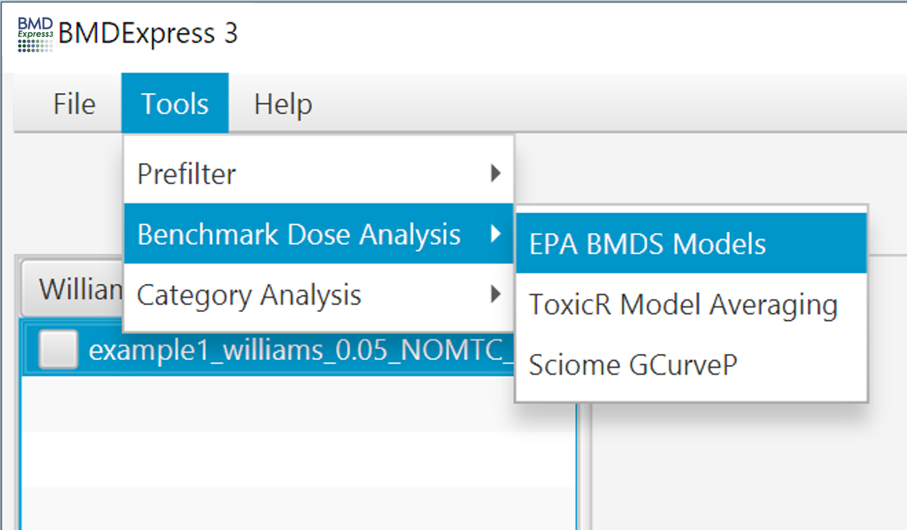
To perform BMD computations, select complete or filtered data set(s) from the Data Selection Area, and click Tools > Benchmark Dose Analysis. Then choose either EPA BMDS Models, ToxicR Model Averaging, or Sciome GCurveP (Non-parametric).

Menu BMD

Video describing Benchmark Dose Analysis setup

Document describing model inputs and outputs, and of the best model selection work flow

Document describing GCurveP method and work flow

IMPORTANT:

BMDExpress 3 is available for Windows, Mac and Linux operating systems, however BMD results may vary to a small extent across these operating systems due floating point calculations having some variability across code compiled for different platforms. Empirical evaluation of the differences across platforms indicate there are minimal changes to the results, however the results from a limited number of probes may change significantly.

ToxicR model averaging (MA)

ToxicR MA is a Bayesian model averaging (BMA) approach that applies Bayesian inference to model selection and combines estimation across multiple models by averaging across models. When using the Bayesian approach to model fitting, we define priors that place low prior probability on model fits of low plausibility. Once individual model fits are obtained, BMA averages are based on posterior probabilities across models. Model averaging is rapidly becoming the preferred method for performing dose-response modeling with number regulatory organizations including NIOSH, WHO and EFSA indicating their support for the use of model averaging approaches.

Popup BMD

ToxicR MA Data Options

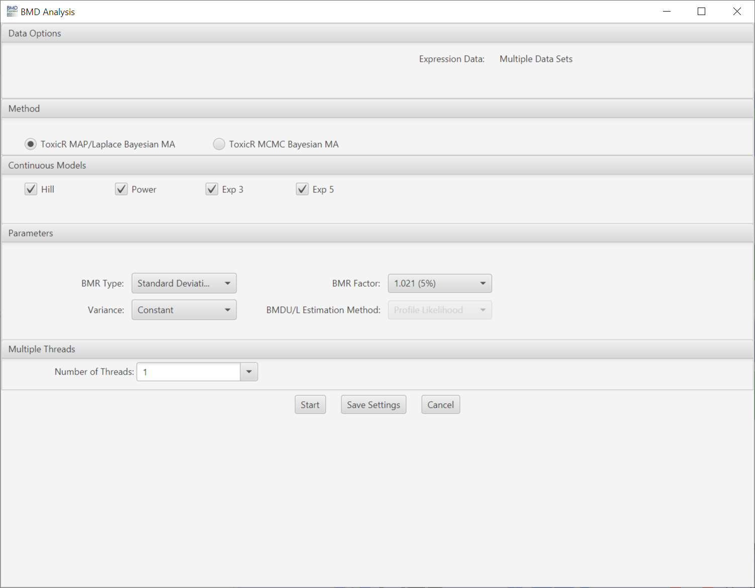
Lists expression data and any pre-filtering in the current workflow.

ToxicR MA Method

ToxicR MAP/Laplace Bayesian MA: This approach to model averaging uses maximum a-posteriori estimation (MAP), which uses the mode of the posterior distribution as the parameter estimate. Laplace approximations to the posterior are then used for constructing confidence bounds.
ToxicR MCMC Bayesian MA: This approach employs Markov chain Monte Carlo for estimating model parameters and confidence intervals.
In both situations (Laplace and MCMC), posterior model probabilities are estimated using the Laplace approximation to the posterior weights. These values can be thought of as the posterior belief that the model is true given the data.
The Laplace and MCMC Bayesian model averaging approaches employed in BMDExpress 3 are taken from the corresponding modeling approaches in package ToxicR package. The ToxicR modeling package and associated methods has undergone peer review and has been published. The statistical/mathematical basis of the ToxicR model averaging approach has also been published.

Continuous Models used in ToxicR model averaging

Choose model(s) for curve fitting. Some of the models will be selected by default. The number of polynomial models available is automatically determined by the unique number of doses comprising the dose-response data. Any single model or combination of models may be chosen.

Model Equations for continuous models implemented in ToxicR (BMDS 3) are shown below, and described in greater depth in the NIEHS White Paper. For all equations, µ is the mean response predicted by the model.

Hill model: μ(dose)=γ+ (v dose^n)/(k^n+ dose^n )
Power model: μ(dose)=γ+ β dose^δ where 0 < γ < 1, β ≥ 0, and 18 ≥ δ > 0.
Exponential 3: μ(dose)=a*exp⁡(sign* (b*dose)^d)
Exponential 5: μ(dose)=a*(c-(c-1)*exp⁡(-1* (b*dose)^d ))

ToxicR Model Averaging Parameters

Variance: Choose whether to use constant or non-constant variance in the modeling.
BMR Factor: Also called the benchmark response or critical effect size in some publications, the number of standard deviations at which the BMD is defined. The BMR is defined relative to the response at control. Since both the response at control and the standard deviation used to calculate the BMR are parameters estimated as part of the curve fit, the BMR may change when the model used to fit the data changes. The recommended default BMR factor is 1 (equivalent to 1 standard deviation), consistent with EPA recommendations for continuous data.
BMDU/L Estimation Method:

EPA BMDS models

Popup BMD

EPA BMDS Data Options

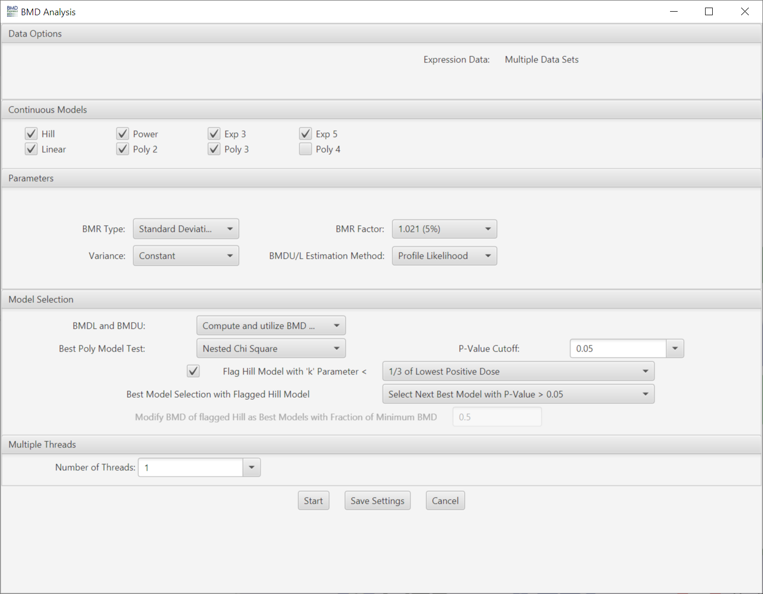
Lists expression data and any pre-filtering in the current workflow.

EPA BMDS Method

This method entails first fitting multiple parametric maximum likelihood estimate (MLE) models to the data, then selecting the single best model that describes the data and determining the estimated BMD, BMDL and BMDU values. In depth descriptions of these models and the model selection approach/criteria can be found in the EPA BMDS guidance document

EPA BMDS Continuous Models

Choose model(s) for curve fitting. Some of the models will be selected by default. The number of polynomial models available is automatically determined by the unique number of doses comprising the dose-response data. Any single model or combination of models may be chosen.

Model Equations for continuous models implemented in BMDExpress 3 are shown below, and described in greater depth in the EPA BMDS 3 User Information site. For all equations, µ is the mean response predicted by the model.

Hill model: μ(dose)=γ+ (v dose^n)/(k^n+ dose^n )
Power model: μ(dose)=γ+ β dose^δ where 0 < γ < 1, β ≥ 0, and 18 ≥ δ > 0.
Exponential 3: μ(dose)=a*exp⁡(sign* (b*dose)^d)
Exponential 5: μ(dose)=a*(c-(c-1)*exp⁡(-1* (b*dose)^d ))
Poly N model: μ(dose)=β_0+β_(1) dose+ β_(2) dose^2+ ⋯ + β_(N) dose^N where N is the degree of the polynomial.
Linear model: The linear model is a special case of the polynomial model with N fixed at 1.

Note: For the the exponential models, "sign" is the adverse direction

Note2: Unlike BMDExpress2, BMDExpress3 allows the modeling of data with single replicates at each dose level and all models are tolerant of negative values, hence it is now possible to model control ratio/subtracted data

EPA BMDS Parameters

Curve fitting is performed using methods implemented in the U.S. Environmental Protection Agency’s BMDS and also found in ToxicR. Adverse direction is determined automatically in the curve fitting computation (i.e., determined by the linear trend test embedded in the model). Parameters that cannot be altered by the user are: benchmark response (BMR) type (set to Std Dev), relative function convergence (set to 1e-8), parameter convergence (set to 1e-8), BMDL curve calculation (set to 1), BMDU curve calculation (set to 1) and smooth option (set to 0).

BMR Type: Standard deviation or relative deviation.
Variance: Choose whether constant or non-constant variance is used in the modeling.
BMR Factor: Also called the benchmark response or critical effect size in some publications, the number of standard deviations at which the BMD is defined. The BMR is defined relative to the response at control. Since both the response at control and the standard deviation used to calculate the BMR are parameters estimated as part of the curve fit, the BMR may change when the model used to fit the data changes. The recommended default BMR factor is 1 (equivalent to 1 standard deviation), consistent with EPA recommendations for continuous data.
BMDU/L Estimation Method: Two options for estimating the upper and lower bounds of the BMD. The EPA preferred method is "profile likelihood" which is computationally and mathematically more rigorous. The second method is the Wald method which is computationally more efficient but is considered less mathematically rigorous. The use of the Wald method is in part what made the FastBMD software faster than previous versions of BMDExpress. For more discussion on the topic the readers are referred to Ren and Xia, 2019 and references there in.
Monotonic Poly2: Checking the box constrains the Poly2 model to being monotonic
Step Function Threshold: Identifies models that change between any two dose levels at or more than the fraction of the total response selected by the user. For example, a value of 0.6 would identify curve fits that change between two dose levels by an amount equal to or greater than 60% of the total response across the entire study. This can be used to identify implausible (i.e. step function) fits to the data, which can then be removed in subsequent analysis steps. Values between 0.5 and 0.6 are typically effective for identifying implausible fits. However, caution should be exercised when applying the step function threshold to studies with five or fewer dose levels. Specifically, it is advisable to visually inspect the fitted data to ensure that probes with plausible responses or fits are not inadvertently removed when applying the step function as a filter in subsequent analyses. Additionally, when using the step function threshold, it is important to verify that the dose range for the study was appropriate. That is, the dose range should have been low enough to capture all plausible responses. If a plausible dose with no transcriptional effect was not achieved, the application of the step function threshold might incorrectly identify true responses as step functions at the lower end of the dose-response curve. These may inadvertently be removed later in the analysis if the step function threshold is used as a filter.

EPA BMDS Model Selection

BMDL and BMDU: Statistical lower and upper bounds on the computed benchmark dose. Choose whether to compute, and whether to include in best model selection criteria.
Best Poly Model Test:
- Nested Chi Square: A nested likelihood ratio test is used to select among the linear and polynomial (2° polynomial, 3° polynomial, etc.) models followed by an Akaike information criterion (AIC) comparison (i.e., the model with the lowest AIC is selected) among the best nested model, the Hill model and the power model.
- Lowest AIC: A completely AIC-based selection process is performed.
P-Value Cutoff: Statistical threshold for the Nested Chi Square test when selecting the best linear/poly model
Flag Hill Model with ‘k’ Parameter < : If the Hill model is selected as one of the models to fit the data, flag a Hill model if its ‘k’ parameter is smaller than the lowest positive dose, or a fraction (1/2, or 1/3) of the lowest positive dose. This option is included since the Hill model can provide unrealistic BMD and BMDL values for certain dose response curves even when it provides the lowest AIC value.
Best Model Selection with Flagged Hill Model: For flagged Hill models, there are multiple options when selecting the best model:
- Include Flagged Hill Models: There is no additional condition applied when selecting the best model.
- Exclude Flagged Hill from Best Models: The flagged Hill model will not be considered when selecting the best model.
- Exclude All Hill from Best Models: All Hill models, either flagged or not, will not be considered when selecting the best model.
- Modify BMD if Flagged Hill as Best Model: If a flagged Hill model is selected as the best model, then modify its BMD value based on a defined fraction of the lowest BMD from the feature/probe set in the data set with a non-flagged Hill model as the best fit model. Note: With this option the user will need to enter a value in the "Modify BMD of flagged Hill as Best Models with Fraction of Minimum BMD". The default value for this parameter is 0.5. Warning: we do not recommend doing this if the object is to identify individual feature or gene BMD values because this can provide an inaccurate estimate of potency.
- Select Next Best Model with P-Value > 0.05: The next best model will be selected that meets both the minimum AIC value and a goodness-of-fit p-Value > 0.05. If another model can not be identified to replace the flagged Hill model a BMD, BMDL and BMDU value is assigned to the probe that equals 0.5*the lowest BMD, BMDL and BMDU of the best models after excluding the flagged Hill models.

EPA BMDS Multiple Threads

Number of threads: This option allows the user to perform multiple model fit computations in parallel by utilizing multiple CPU cores. The option increases the efficiency of CPU usage and significantly reduces the computational time. For example, a computer with a quad-core processor will theoretically require 1/4^th the time to complete model fitting when 4 threads are selected rather than 1 thread. In practice, the actual efficiency varies. Try different values to optimize in your particular situation. Open a processor monitoring utility, and observe processor utilization. Typically, utilization of >80% can be achieved when setting the number of threads to be several to 10-fold greater than the number of processor cores. The default recommendation for the number of threads is 4 times the number of cores that are available. The recommendation is less than this if the user plans to carry out additional computational tasks while modeling is being performed.
- N.B. increasing processor utilization by BMDExpress will hinder interactive responsiveness.

After selecting and checking the appropriate data, models, parameters, and other options, click Start. Computation may take minutes to hours depending on the total number of probe set identifiers and data sets submitted for analysis, the number of models to fit, and your computer’s performance characteristics.

Benchmark Dose Data Options (Sciome GCurveP)

Statistical outliers in the dose-response data can result in a non-monatonic curve fit. Some users interpret this as an unrealistic outcome. GcurveP is a non-parametric curve correction algorithm that is based on the assumption that the correct dose-response curve must exhibit monotonic behavior. It finds a minimal set of corrections needed to restore monotonic behavior of the dose-response curve. It takes the direction of monotonicity (i.e., ascending, flat, or descending) as its input parameter, and iteratively searches from each dose-group of the curve, as its trusted pivot point, for monotonicity violations. It then counts how many other curve points would need adjustments (i.e., by shifting respective dose groups) to restore monotonicity. The final solution is then the set with minimal number of such points that require corrections.

Popup BMD GCurveP

Data Options

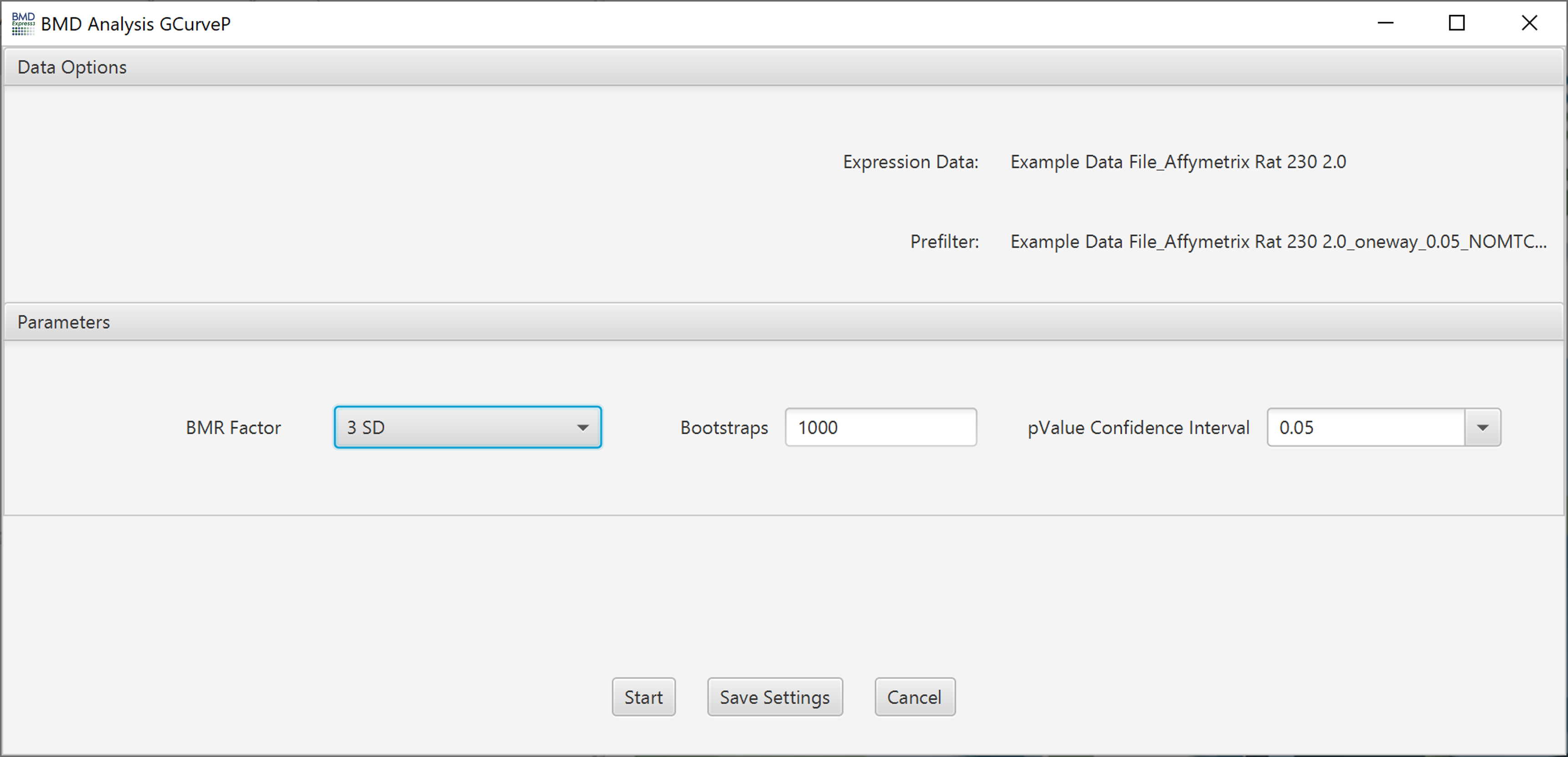
Lists expression data and any pre-filtering in the current workflow.

Parameters

BMR Factor: Also called the benchmark response or critical effect size. It is a multiple of standard deviation (SD) of the probe/gene expression change relative to its expression level at control. It determines the change in expression at which the BMD is defined. We recommend setting a BMR Factor to 3 when using GCurvep because it uses an adjusted standard deviation that down weights outlier values that leads to a compression of the estimated SD.
Bootstraps: Monotonicity correction is repeated by a bootstrap sampling algorithm. 1000 times is the default.
pValue Confidence Interval: Default is 0.05, which means the software will calculate a 95% confidence interval

Multiple Threads

Number of Threads: Not yet implemented.

Benchmark Dose Results

Video describing Benchmark Dose Analysis results

Main BMD results

Results are tabulated in the bottom half of the window:

Probe ID: Unique identifier for probe/probe set ID.
Genes: All genes included in probe/probe set.
Gene Symbols: Gene symbols included in probe/probe set.

When BMDS is used for curve fitting, there are columns for the "Best" model, and the other models that were computed.

Click to show list of result columns.

BMD: Benchmark dose
BMDL: Lower bound of the 95% confidence interval of the benchmark dose
BMDU: Upper bound of the 95% confidence interval of the benchmark dose
fitPValue: Global goodness of fit (GGOF) measure. Small p-values indicate that the model is a poor fit to the data. More specifically, the model identified by AIC is further compared with the dose response from fully saturated model (unconstrained model that is free from any functional form or trajectory constraints) using conventional likelihood ratio test statistic. The larger p-value for this test indicates that the identified model is not statistically inferior fit than the saturated model, whereas the smaller p-value indicates that the identified model does not fit the data as well as the saturated model and hence it is possible to device a better fitting model. Note: All dose groups must have atleast an n=2 to allow for a fit p-value to be calculated. If any dose group has n=1 then the fit p-value will be reported as "0".
fitLogLikelihood: A value calculated using the log of the likelihood given the model, used in calculating the AIC. The value is used to compare between different model fits to the same feature.
AIC: Akaike Information Criterion. Given a set of dose-response models for a probe set/gene the AIC estimates the quality of each model relative to the other models. In most cases with BMDExpress the model with the lowest AIC is selected as the "best model".
adverseDirection: Direction of the dose-response (i.e., up- or down-regulation) as identified by the software
BMD/BMDL Ratio
BMDU/BMDL Ratio
BMDU/BMD Ratio
Prefilter P-Value: statistical cutoff in probe selection step
Prefilter Adjusted P-Value: statistical cutoff in probe selection step, with adjustment applied
Max Fold Change: maximum fold change of all probes selected for BMD computation
Max Fold Change Absolute Value
NOTEL: No Observed Transcriptional Effect Level; highest dose that does not cause a transcriptional change in a transcript/gene.
LOTEL: Lowest Observable Transcriptional Effect Level; lowest dose resulting in transcriptional change in a transcript/gene.
FC Dose Level <n>: fold change at each dose level n
Flagged: Value = "1" indicates that the Hill model was flagged for that probe or gene based on the setting selected in the BMD analysis set up. "0" indicates the Hill model was not flagged
Model Residual 1-x: abs (Dose group average value-model value at dose level). Used to calculate coefficient of determination (Rsquared)
Model RSquared: Coefficient of determination. An alternative metric to the GGOF p-value for evaluation of model fit to the data. Models with values >0.6 typically show acceptable fits upon visual inspection.
Model is Step Function: Indicates that the model exhibits step function change > predefined fraction, i.e., the model the model changed between any 2 dose groups is > the predefined fraction in the BMD modeling set up
Model is Step Function With Step Function Less Than Lowest Dose: Indicates that the model exhibits step function change > predefined fraction between the first (typically vehicle) and the second dose (usually the lowest non-0 dose), i.e., the model the model changed between the vehicle and fist dose level is > the predefined fraction in the BMD modeling set up
For each model fit to the data, specific parameters for each probe set/gene are reported. This is done to allow the user to recapitulate the model equations.
There is also a corresponding set of columns for the "Best" fit model (i.e., BMD, BMDL, BMDU, fitPValue, fitLogLikeihood, AIC, BMD/BMDL, BMDU/BMDL, Prefilter P-value, Prefilter Adjusted P-value, Max Fold Change, Max Fold Change Absolute value),
FC Dose Level n: Fold change at dose n.

For a more detailed definition of terms please refer to the EPA BMDS User Guide

With GCurveP, there are columns similar to the BMDS models, plus GCurveP-specific results:

Click to show GCurveP results list.

- **fitValue:** fraction of original signal preserved after GCurveP treatment - **Excecution Complete:** true or false; indicates whether computation completed under the selected initial conditions

And, for ToxicR MA, there are columns similar to the MLE/BMDS models, plus specific results relates to Bayesian modeling and averaging:

Click to show Bayesian MA results list.

MA BMD: Model average BMD
MA BMDL: Model average BMDL
MA BMDU: Model average BMDU
MA adverseDirection: Model average direction of change (i.e., does the dose-response curve show an increasing or decreasing trend)
MA BMD/BMDL: BMD/BMDL ratio of the average model
MA Execution Complete: Indicates if model averaging was successfully completed
MA Hill Posterior Probability: the posterior probability of the hill model
MA Power Posterior Probability: the posterior probability of the power model
MA Exp 3 Posterior Probability: the posterior probability of the exp3 model
MA Exp 5 Posterior Probability: the posterior probability of the exp5 model
Note: the "best" results (e.g. Best BMD) when using the BMA are the same as the model average results

Curve Viewer

Each probeset ID is a hyperlink to a separate window that displays a plot of the corresponding dose response behavior and model fit curves.

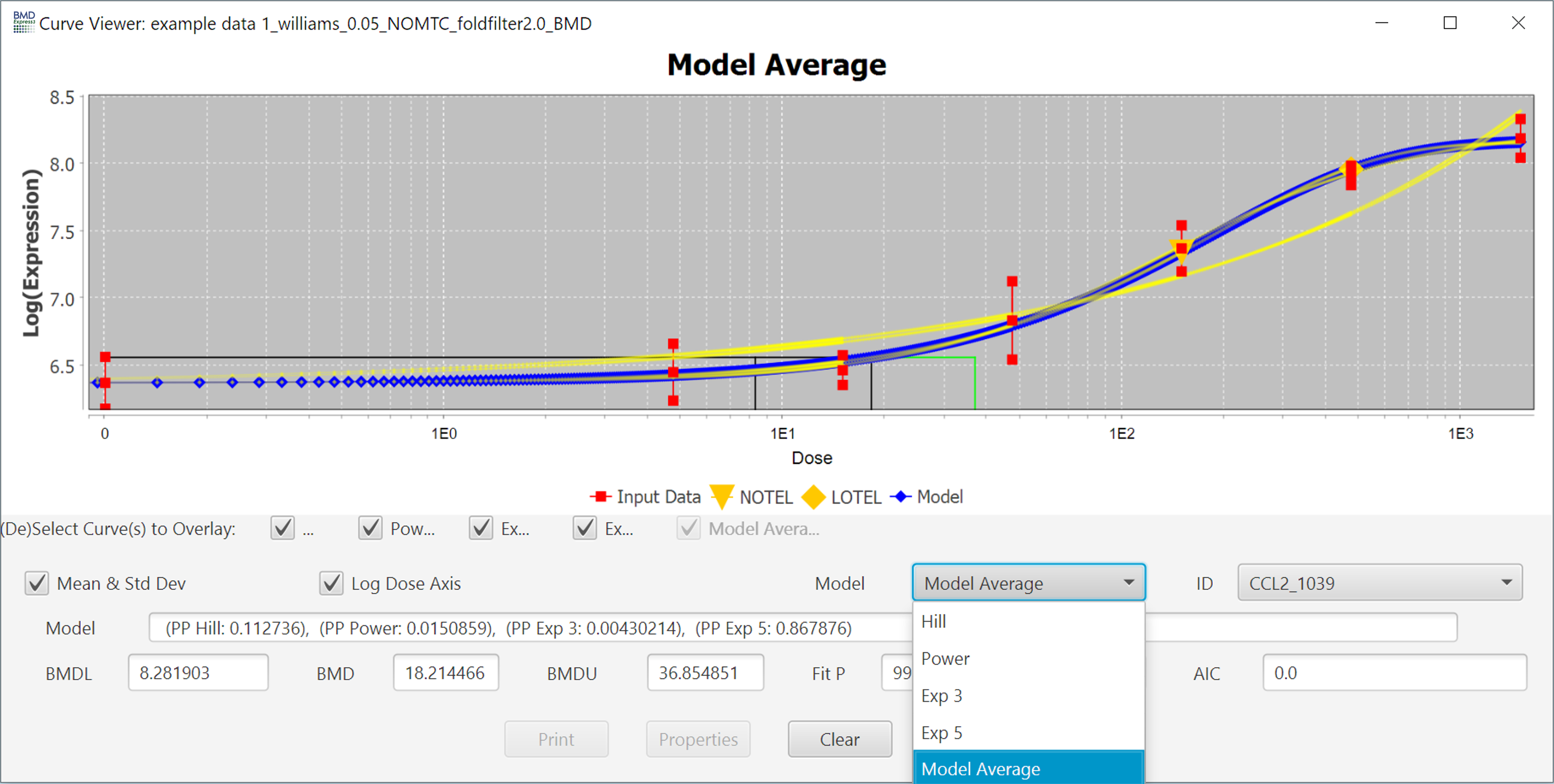
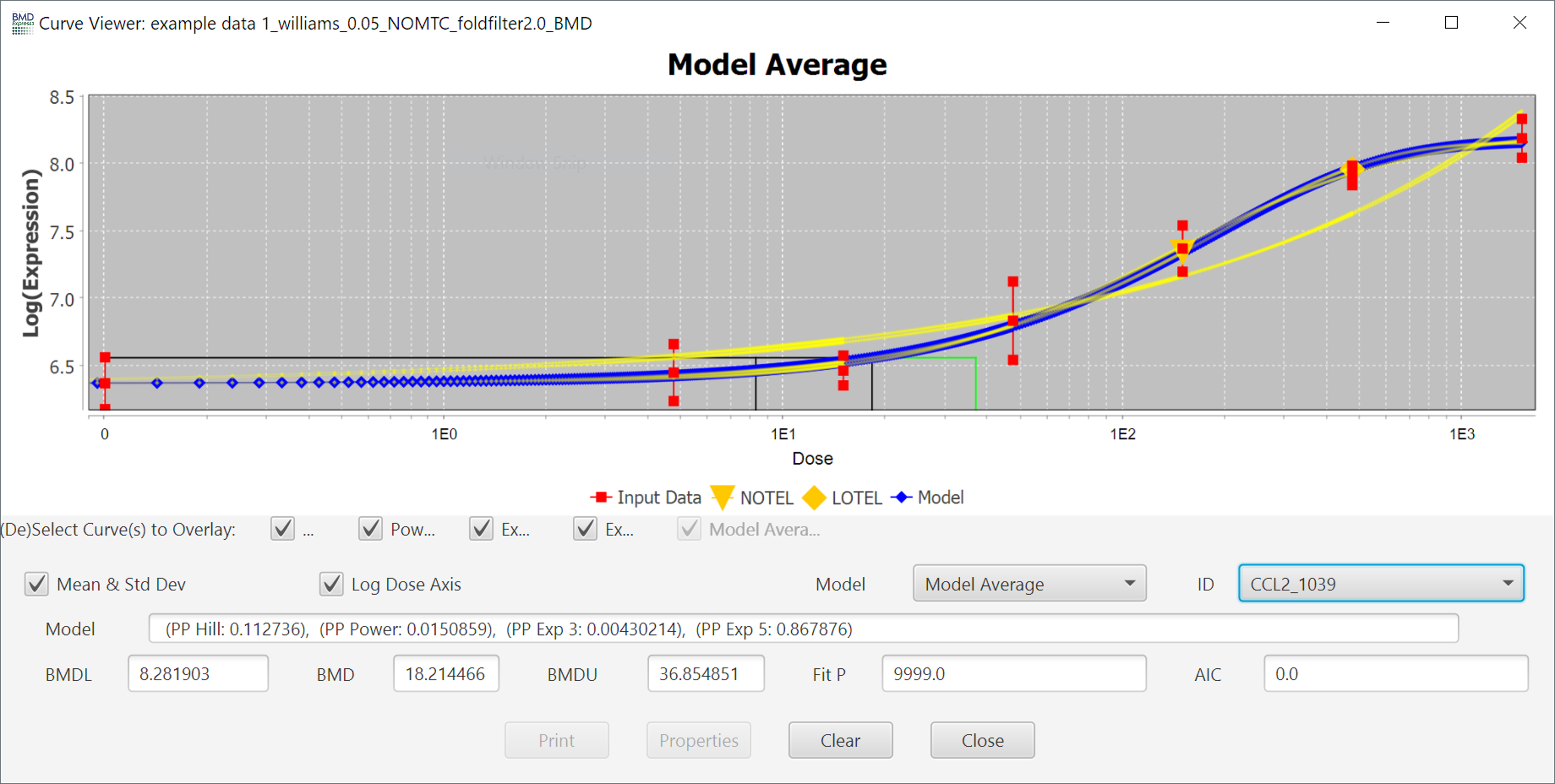Popup curve The curve that is shown initially is the one with the best fit as described in the introduction, but you can view the fit of other models by using the Model dropdown menu.

Popup curve model

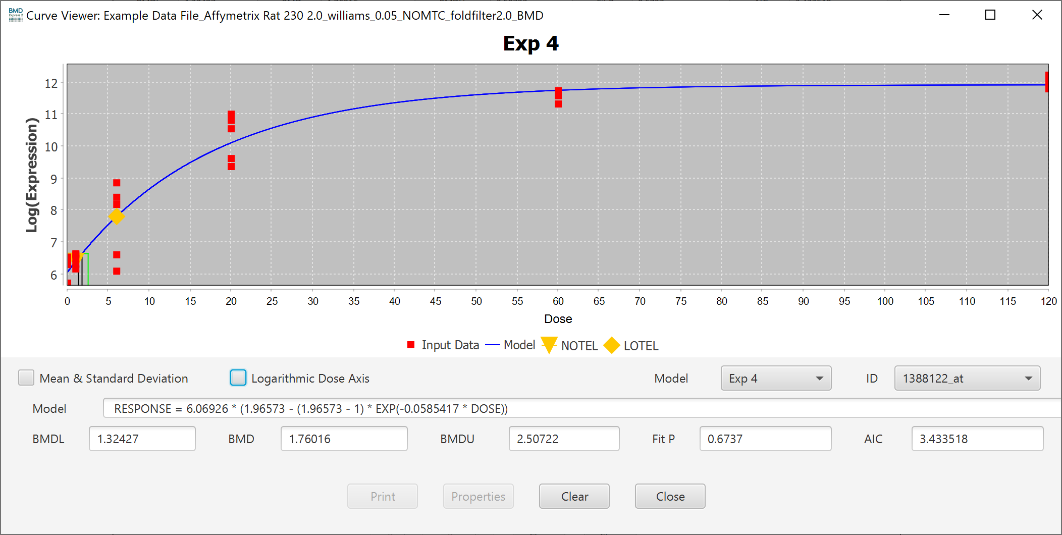
The Mean & Standard Deviation checkbox toggles the points in the plot to reflect the mean and standard deviation of each dose, or the response data points.

Popup curve mean SD

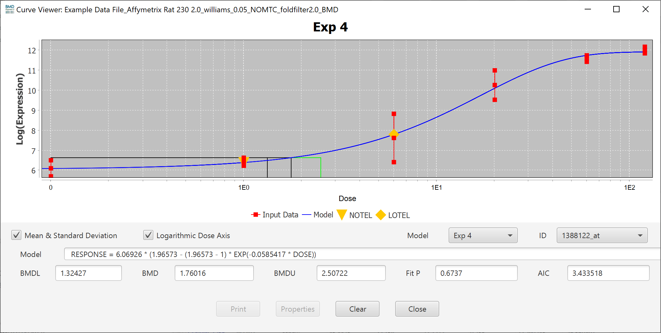
You can also change the scale of the axis to linear by unchecking the Logarithmic Dose Axis checkbox.

Popup curve log

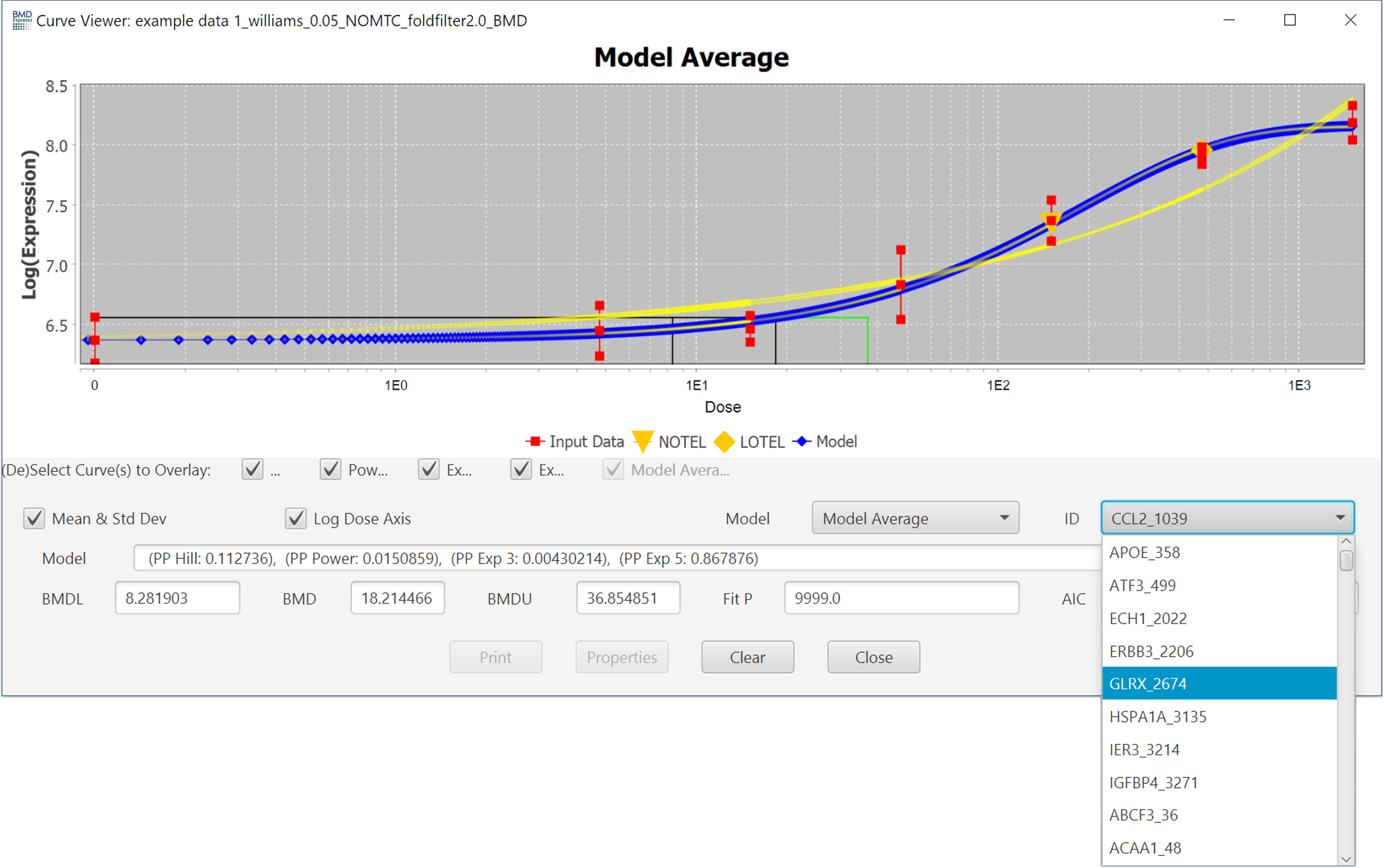
You can switch between different probes/probe sets inside of the individual curve viewer using the ID dropdown, however it is usually faster to close the popup and double-click on a different probe/probe set in the results table.

Popup curve ID

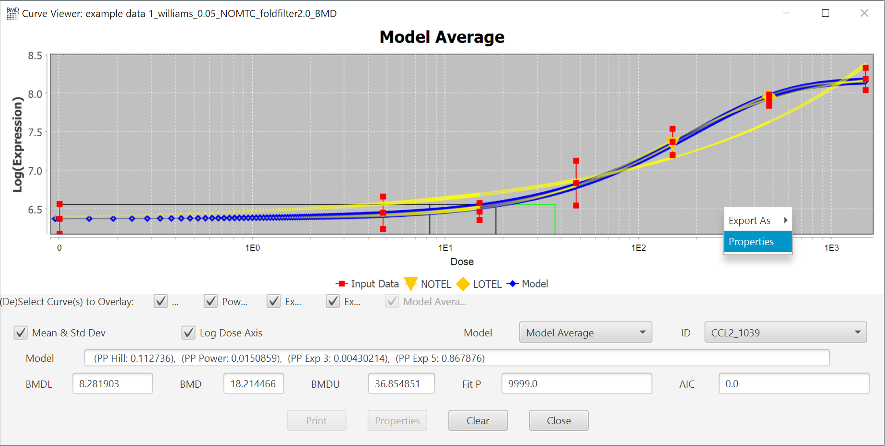
All properties of the curve can be altered in the Properties Menu, accessed by right-clicking in the chart area.

Popup curve properties

Inside the Chart Editor for the plot, there are a variety of parameters that can be changed to alter the appearance of the plot.

Title
- Show Title
- Title Text
- Font
- Color
Plot
- Domain & Range Axis
  - Label
  - Font
  - Paint
- Other
  - Ticks
    - Show tick labels
    - Tick label font
    - Show tick marks
  - Range
    - Auto-adjust range
    - Minimum range value
    - Maximum range value -TickUnit
    - Auto-selection of TickUnit
    - Tickunit Value
- Appearance
  - Outline Stroke
  - Outline Paint
  - Background Paint
  - Orientation
Other
- Draw anti-aliased
- Background paint
- Series Paint
- Series Stroke
- Series Outline Paint
- Series Outline Stroke

Finally, you export an image of the plot by right clicking on the image and selecting "Export As" and then selecting the image file format.

Benchmark Dose Visualizations

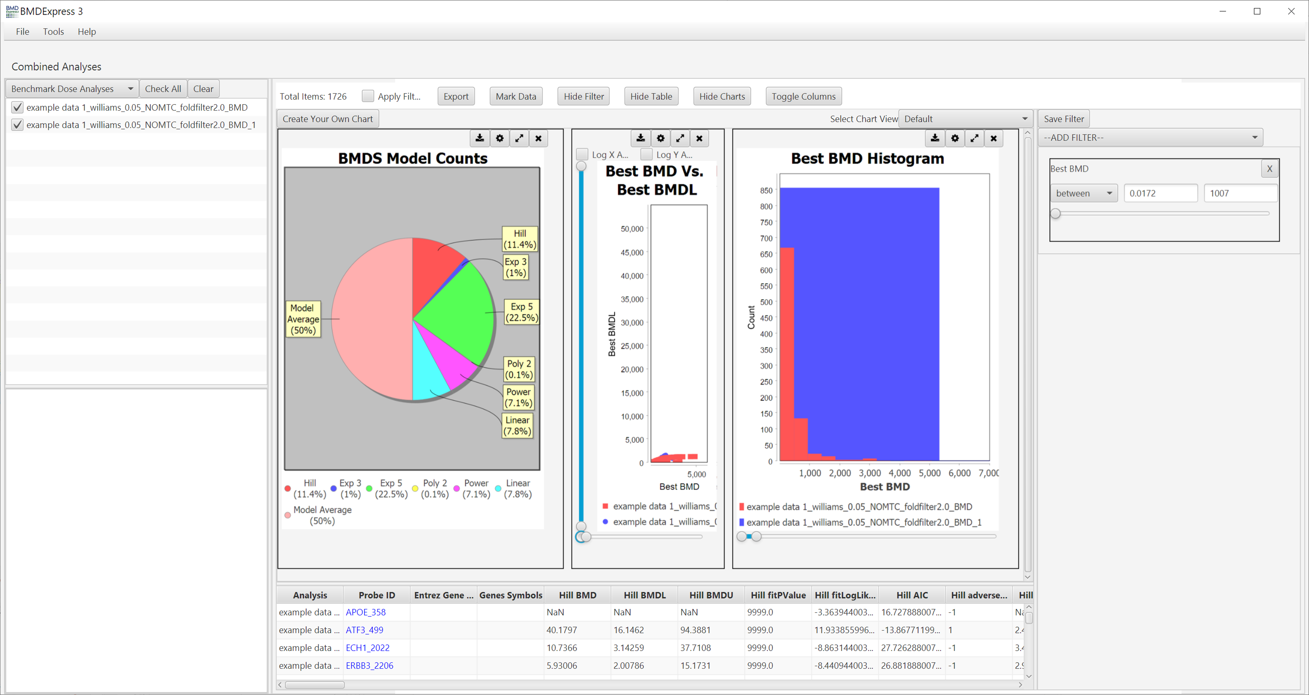
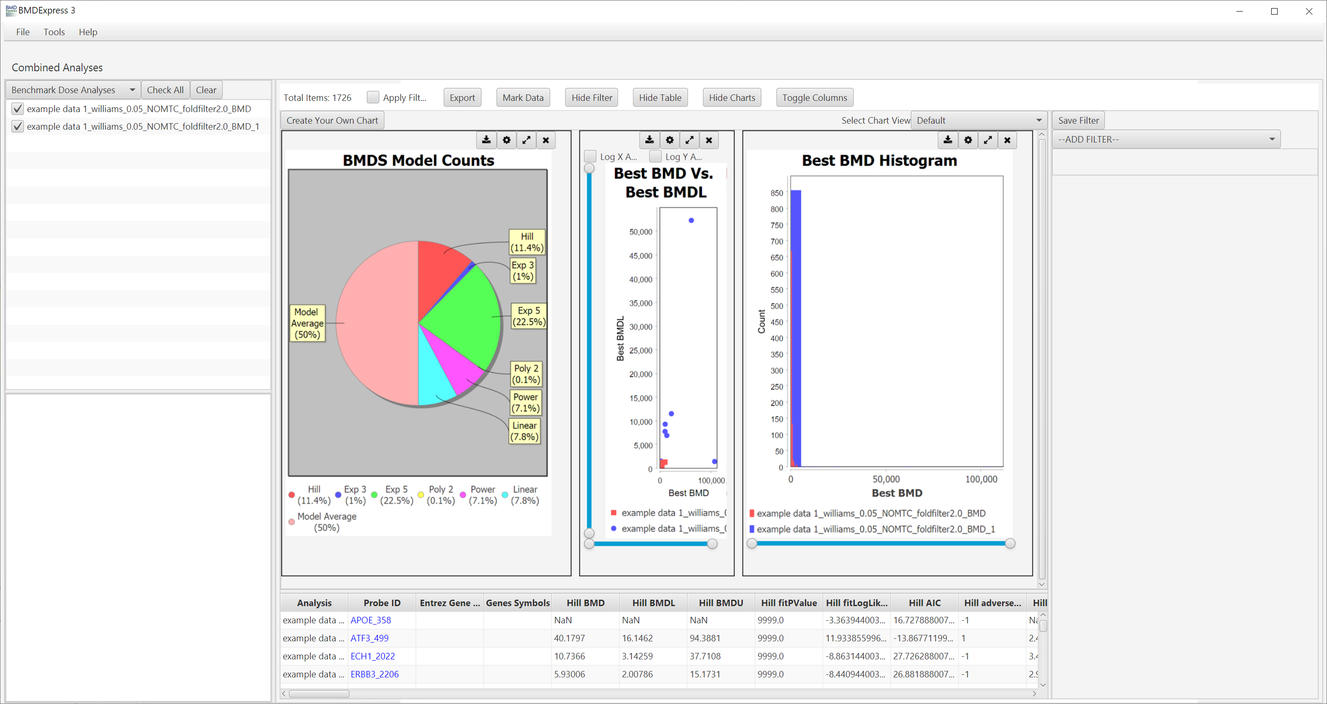
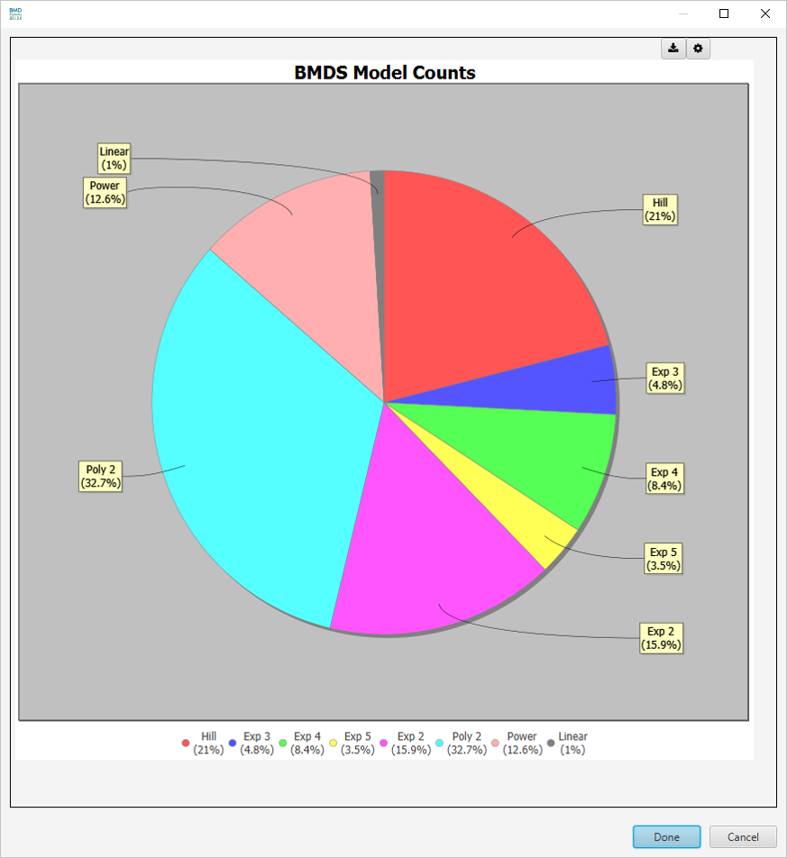
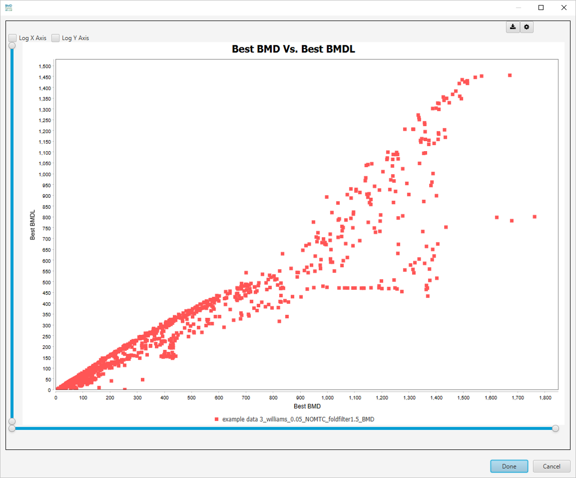
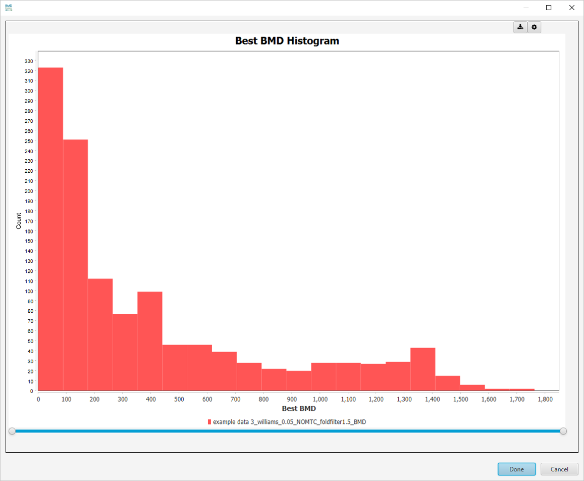
The default visualizations are:

BMDS Model Counts
Best BMD Vs. Best BMDL
Best BMD Histogram

Additional visualizations are available by making a selection in the Select Graph View dropdown list.