wrapper_primer
This document assumes that adda is installed and available at the command line under ../adda/src/seq/adda (to be modified as appropriate). A basic wrapper creates a command line that is passed to the shell, executed, and the results (cross-sections) are captured internally; all being done within R.
First, we load some helpful libraries.
library(dielectric) # dielectric function of Au and Ag
library(plyr) # convenient functions to loop over parameters
library(reshape2) # reshaping data from/to long format
library(ggplot2) # plotting frameworkadda_spectrum <- function(shape = "ellipsoid",
euler = c(0, 0, 0),
AR = 1.3,
wavelength = 500,
radius = 20,
n = 1.5 + 0.2i ,
medium.index = 1.46,
dpl = ceiling(min(50, 20 * abs(n))),
test = TRUE, verbose=TRUE, ...) {
command <- paste("echo ../adda/src/seq/adda -shape ", shape, 1/AR, 1/AR,
"-orient ", paste(euler, collapse=" "),
"-lambda ", wavelength*1e-3 / medium.index ,
"-dpl ", dpl,
"-size ", 2 * radius*1e-3,
"-m ", Re(n) / medium.index ,
Im(n) / medium.index , ...)
if(verbose)
message(system(command, intern=TRUE))
if(test) return() # don't actually run the command
# extract the results of interest
resultadda <- system(paste(command, "| bash"), intern = TRUE)
Cext <- as.numeric(unlist(strsplit(grep("Cext",resultadda,val=T)[1:2],s="="))[c(2,4)])
Cabs <- as.numeric(unlist(strsplit(grep("Cabs",resultadda,val=T)[1:2],s="="))[c(2,4)])
Csca <- Cext - Cabs
c(Cext[1], Cext[2], Cabs[1], Cabs[2], Csca[1], Csca[2])
}
# testing that it works
adda_spectrum(test = FALSE)## ../adda/src/seq/adda -shape ellipsoid 0.769230769230769 0.769230769230769 -orient 0 0 0 -lambda 0.342465753424658 -dpl 31 -size 0.04 -m 1.02739726027397 0.136986301369863
## [1] 9.826e-05 1.008e-04 9.808e-05 1.006e-04 1.759e-07 1.819e-07
We first define a wavelength-dependent dielectric function for the scatterer, here gold in the visible region. A loop is then performed over the wavelengths; the cross-sections are stored in a matrix, and plotted at the end.
gold <- epsAu(seq(400, 700, length=100))
str(gold)
## 'data.frame': 100 obs. of 2 variables:
## $ wavelength: num 400 403 406 409 412 ...
## $ epsilon : cplx -1.65+5.77i -1.67+5.78i -1.68+5.79i ...
## empty matrix to store the results
results <- matrix(ncol=6, nrow=nrow(gold))

## loop over the wavelengths
for( ii in 1:nrow(gold) ){
  results[ii, ] <- adda_spectrum(wavelength = gold$wavelength[ii],
                                 n = sqrt(gold$epsilon[ii]),
                                 radius = 20, AR = 1.3, dpl=50,
                                 test = FALSE, verbose = FALSE)
}

str(results)
## num [1:100, 1:6] 0.00128 0.00127 0.00126 0.00125 0.00124 ...
## basic plot
matplot(gold$wavelength, results,
        type = "l", col = rep(1:3, each=2),
        lty = rep(1:2, 3),
        xlab = "Wavelength /nm",
        ylab = expression("Cross-sections /"*nm^2),
        main = "Au ellipsoid")

legend("topleft", legend=expression(sigma[ext],sigma[abs],sigma[sca], "",
                                     "x-polarisation", "y-polarisation"),
       inset=0.01, col=c(1:3, NA, 1, 1), lty=c(1,1,1, NA, 1, 2),
       bg  = "grey95", box.col=NA)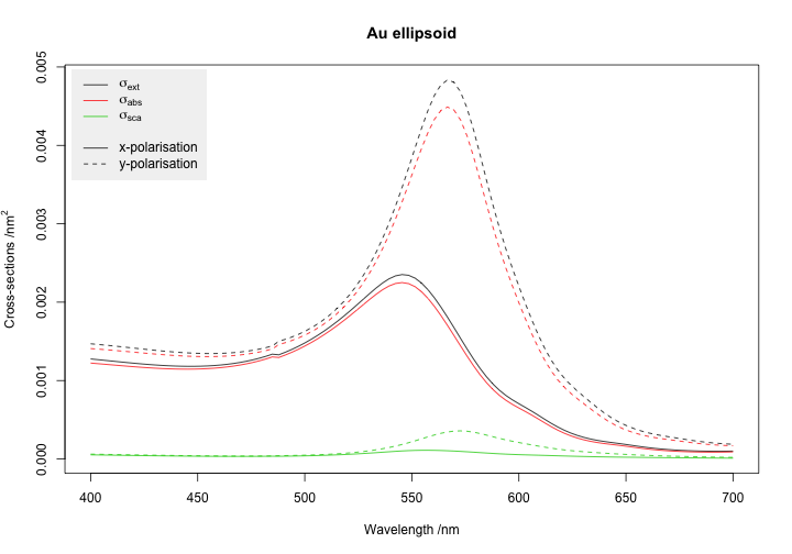
We define a convenience function to run a simulation (full spectrum), with a specific value of particle size and aspect ratio. Instead of using an explicit for loop, we use a very convenient package plyr which defines functions such as mdply to encapsulate for loops in a more expressive and succint notation.
Note that to keep the simulation short, -dpl is kept too small to ensure a reliable result for the cross-sections.
gold <- epsAu(seq(400, 700, length=200))

simulation <- function(radius = 20, AR = 1.3, ..., material=gold){
  params <- data.frame(wavelength = material$wavelength,
                       n = sqrt(material$epsilon),
                       radius = radius,
                       AR = AR)
  results <- mdply(params, adda_spectrum, ..., test=FALSE)

  # reshape the data from wide to long format
  m <- melt(results, measure.vars = c("V1","V2","V3","V4","V5","V6"))

  # create new ID columns to keep track of polarisation and type
  m$polarisation <- m$type <- factor(m$variable)
  levels(m$polarisation) <- list(x = c('V1','V3','V5'),
                                 y = c('V2','V4','V6'))
  levels(m$type) <- list(extinction = c('V1','V2'),
                         absorption = c('V3','V4'),
                         scattering = c('V5','V6'))
  m
}

test <- simulation(radius = 20, AR = 1.3, verbose = FALSE)
str(test)
## 'data.frame': 1200 obs. of 8 variables:
## $ wavelength : num 400 402 403 405 406 ...
## $ n : cplx 1.48+1.96i 1.47+1.96i 1.47+1.96i ...
## $ radius : num 20 20 20 20 20 20 20 20 20 20 ...
## $ AR : num 1.3 1.3 1.3 1.3 1.3 1.3 1.3 1.3 1.3 1.3 ...
## $ variable : Factor w/ 6 levels "V1","V2","V3",..: 1 1 1 1 1 1 1 1 1 1 ...
## $ value : num 0.00128 0.00127 0.00127 0.00126 0.00126 ...
## $ type : Factor w/ 3 levels "extinction","absorption",..: 1 1 1 1 1 1 1 1 1 1 ...
## $ polarisation: Factor w/ 2 levels "x","y": 1 1 1 1 1 1 1 1 1 1 ...
qplot(wavelength, value, colour = polarisation,
      facets = ~ type, data = test, geom = 'line')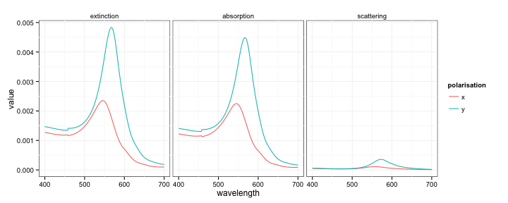
We can very conveniently call this same function with many parameters, and let R collect the results in a single dataset.
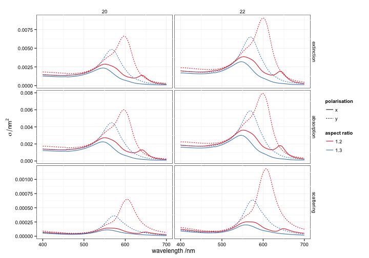
params <- expand.grid(radius = c(20, 22),
                      AR = c(1.2, 1.3))

all <- mdply(params, simulation, verbose = FALSE)

ggplot(all, aes(wavelength, value,
                linetype = polarisation, colour = factor(AR),
                group = interaction(polarisation, AR))) +
  facet_grid(type~radius, scales='free') +
  geom_line() + labs(x = 'wavelength /nm',
                     y = expression(sigma/nm^2),
                     colour = 'aspect ratio') +
  scale_colour_brewer(palette = 'Set1')