Anomaly detection aims to find patterns in databases whose behavior is highly unusual. As a learning task, anomaly detection may be supervised, semi-supervised, or unsupervised. For this assignment we analyzed semi-supervised anomaly detection (SSAD) algorithms, those being Bagging-Random Miner (BRM), Gaussian Mixture Model (GMM), Isolation Forest (ISOF), and One-Class Support Vector Machines (ocSVM). It is worth mentioning that the BRM implementation (Benito Camiña et al. 2019) was modified so it can work with any dissimilarity measure and it was also analyzed using 4 different dissimilarity measures: euclidean distance, correlation distance, cosine distance and manhattan distance.
Consequently, 7 SSAD algorithms were evaluated according to their average AUC score across 93 databases, these being: abalone-3_vs_11, abalone-17_vs_7-8-9-10, abalone-19_vs_10-11-12-13, abalone-20_vs_8-9-10, abalone-21_vs_8, abalone9-18, abalone19, car-good, car-vgood, cleveland-0_vs_4, dermatology-6, ecoli-0_vs_1, ecoli-0-1_vs_2-3-5, ecoli-0-1_vs_5, ecoli-0-1-3-7_vs_2-6, ecoli-0-1-4-6_vs_5, ecoli-0-1-4-7_vs_2-3-5-6, ecoli-0-1-4-7_vs_5-6, ecoli-0-2-3-4_vs_5, ecoli-0-2-6-7_vs_3-5, ecoli-0-3-4_vs_5, ecoli-0-3-4-6_vs_5, ecoli-0-3-4-7_vs_5-6, ecoli-0-4-6_vs_5, ecoli-0-6-7_vs_3-5, ecoli-0-6-7_vs_5, ecoli1, ecoli2, ecoli3, ecoli4, flare-F, glass-0-1-2-3_vs_4-5-6, glass-0-1-4-6_vs_2, glass-0-1-5_vs_2, glass-0-1-6_vs_2, glass-0-1-6_vs_5, glass-0-4_vs_5, glass-0-6_vs_5, glass0, glass1, glass2, glass4, glass5, glass6, habermanImb, iris0, kr-vs-k-one_vs_fifteen, kr-vs-k-three_vs_eleven, kr-vs-k-zero_vs_eight, kr-vs-k-zero_vs_fifteen, kr-vs-k-zero-one_vs_draw, lymphography-normal-fibrosis, new-thyroid1, new-thyroid2, page-blocks-1-3_vs_4, page-blocks0, pimaImbm, poker-8_vs_6, poker-8-9_vs_5, poker-8-9_vs_6, poker-9_vs_7, segment0, shuttle-2_vs_5, shuttle-6_vs_2-3, shuttle-c0-vs-c4, shuttle-c2-vs-c4, vehicle0, vehicle1, vehicle2, vehicle3, vowel0, winequality-red-3_vs_5, winequality-red-4, winequality-red-8_vs_6, winequality-red-8_vs_6-7, winequality-white-3_vs_7, winequality-white-3-9_vs_5, winequality-white-9_vs_4, yeast-0-2-5-6_vs_3-7-8-9, yeast-0-2-5-7-9_vs_3-6-8, yeast-0-3-5-9_vs_7-8, yeast-0-5-6-7-9_vs_4, yeast-1_vs_7, yeast-1-2-8-9_vs_7, yeast-1-4-5-8_vs_7, yeast-2_vs_4, yeast-2_vs_8, yeast1, yeast3, yeast4, yeast5, yeast6, and zoo-3. Each of these datasets were entered into the algorithms with their original values, their values normalized using MinMax scaling, and their values normalized using Standard scaling. The evaluation of the SSAD algorithms are compared and presented in a box plot to visualize the results. With the help of the tool KEEL (I. Triguero et al. 2017) a Friedman test with a Holm post hoc test was performed, we present the results from the 1xN tests where we get the winning algorithm across the 93 datasets and compare it with the other algorithms. We also performed NxN tests from which results a CD diagram was constructed to see which algorithms had statistical differences between them.
The code in the anomaly_benchmark_v3.py file contains the code used to perform the benchmark between the mentioned SSAD algorithms. Here we include the modified class for the modified BRM algorithm which allows the use of any dissimilarity measure. Next we explain each of the functions that can be found there.
raw_train_test_data. This function reads the respective test and train files included in the folder that it receives and returns them. normalization. Receives the raw train and test data and the normalization type, if the type is “no” it returns the same data it receives. If the type is “minmax” it returns the data with a MinMax scaling and if the type is “standard” it returns the data with a standard scaling.
rebuild_preprocessed_train_test. This function takes the preprocessed data and rebuilds it separating the class values from the rest of the features. Then it passes these values to the normalization function and returns the preprocessed and normalized data.
preprocess_dataset. This function takes the raw test and train data, concatenates them and drops the class values, then it separates the nominal and no nominal values and passes to the rebuild_preprocessed_train_test function the nominal values without class to get restructured. model_objects. In this function we create the models that are going to be compared in the benchmark. Here we establish the dissimilarity measures for the modified BRM algorithm.
run_classification_model_brm, run_gmm and run_classification_model_competitor. These functions receive the train and test class values and data, the clf metrics and the model objects that correspond to each algorithm to be tested. They then train and test each model and return the corresponding metrics.
run_all_clf. In this function we get the AUC for all the algorithms and return the results.
normalization_clf_test. Here we read all the datasets included in the folder that we pass to the function, preprocess the datasets and get the AUC for all the algorithms.
export_results. Saves the obtained results in the corresponding folder depending on the algorithm used and the type of normalization.
run_benchmark. Here we start the benchmark process for each type of normalization, we get the results and call the export_results function to save the results.
To generate the boxplots we use the figures.ipynb notebook where we read the results obtained from the benchmark to generate the boxplots of the AUC scores on the datasets with each kind of normalization. The code used for the benchmarking, the generation of the Boxplots, the results obtained from both the testing of the models and the statistical tests as well as the CD diagrams can be found in this repository.
Table 1. Head of the dataset with the AUC scores obtained without normalizing.

Figure 1. Boxplot of the AUC scores on the datasets without normalizing or scaling
- Average rankings of Friedman test
Average ranks obtained by each method in the Friedman test.
Table 2: Average Rankings of the algorithms (Friedman)
Friedman statistic (distributed according to chi-square with 6 degrees of freedom): 66.806452. P-value computed by Friedman Test: 0.
- Adjusted P-values obtained through the application of theHolms post hoc method (Friedman).
Table 3: Adjusted p-values (FRIEDMAN)

Figure 2. CD diagram for the AUC scores on the datasets without normalizing or scaling.
Table 4. Head of the dataset with the AUC scores obtained with MinMax normalization.

Figure 3. Boxplot of the AUC scores on the datasets with MinMax normalization.
- Average rankings of Friedman test
Average ranks obtained by each method in the Friedman test.
Table 5: Average Rankings of the algorithms (Friedman)
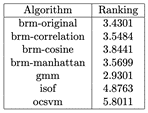
Friedman statistic (distributed according to chi-square with 6 degrees of freedom): 117.470046. P-value computed by Friedman Test: 0.
-Adjusted P-values obtained through the application of theHolms post hoc method (Friedman).
Table 6: Adjusted p-values (FRIEDMAN)
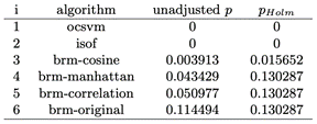
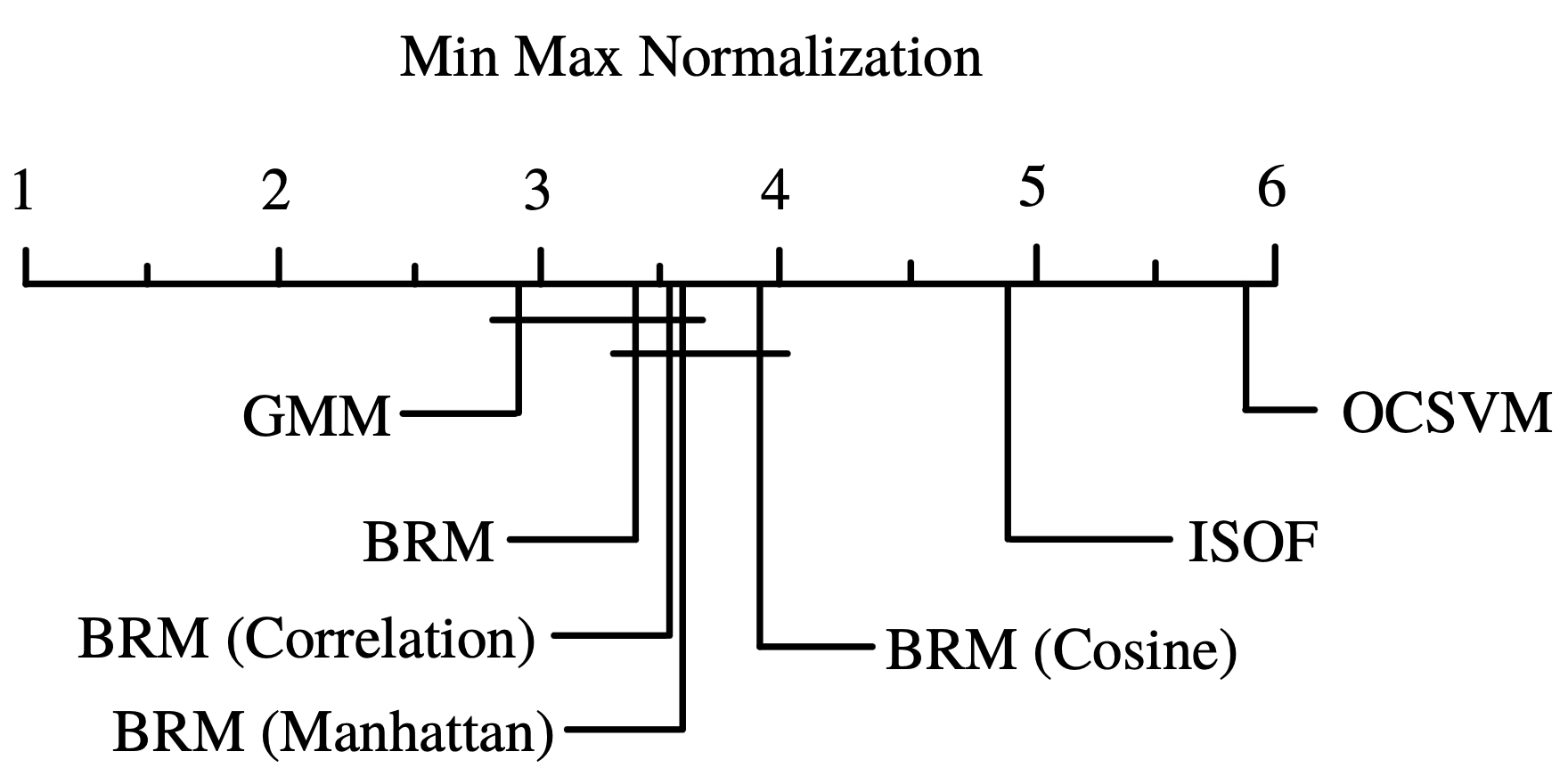
Figure 4. CD diagram for the AUC scores on the datasets with MinMax normalization.
Table 7. Head of the dataset with the AUC scores obtained with MinMax normalization.
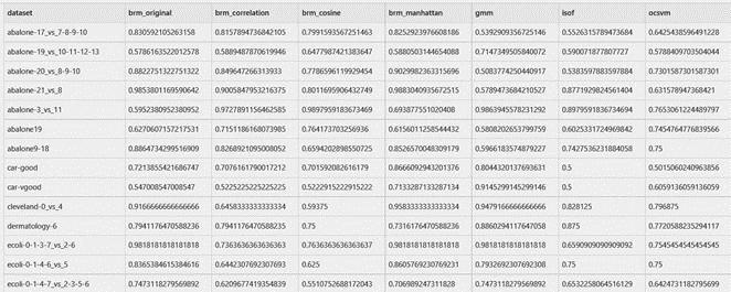
Figure 5. Boxplot of the AUC scores on the datasets with Standard normalization.
- Average rankings of Friedman test
Average ranks obtained by each method in the Friedman test.
Table 8: Average Rankings of the algorithms (Friedman)
Friedman statistic (distributed according to chi-square with 6 degrees of freedom): 96.8053. P-value computed by Friedman Test: 0.
- Adjusted P-values obtained through the application of the Holms post hoc method (Friedman).
Table 9: Adjusted p-values (FRIEDMAN)
Figure 6. CD diagram for the AUC scores on the datasets with Standard normalization.
First we analyzed the AUC results of the algorithms with the datasets without any kind of normalization, we show the head of the resulting cvs in Table 1. We can visualize the resulting AUC in the boxplot from Fig. 1, where we can see that BRM (Manhattan) had the highest AUC median, followed by GMM and BRM. It is worth mentioning that GMM had the highest Q3. Next, in Table 2 we can see the average ranking of the Friedman test for the 1xN tests, which tells us that in this case the winning algorithm was GMM, followed by BRM (Manhattan). Also the Friedman test portrays that between at least 2 algorithms there exists a statistical difference. In Table 3 we see the Holm post hoc comparison results where we test every algorithm against the winning algorithm. Here we are able to notice that BRM (Manhattan) and BRM do not have any statistical difference with the GMM algorithm. Finally, Fig. 2 shows the CD diagram for the AUC scores, we can see that there is no statistical difference between GMM, BRM (Manhattan) and BRM, also between BRM (Manhattan), BRM, BRM (Correlation) and BRM (Cosine), also between BRM (Correlation), BRM (Cosine) and ocSVM and finally between ocSVM and ISOF.
For this section, we analyzed the AUC results of the algorithms with the datasets with MinMax normalization, we show the head of the resulting cvs in Table 4. We can visualize the resulting AUC in the boxplot from Fig. 3, where we can see that GMM had the highest AUC median of all followed by BRM. Also, it is visible that GMM had the highest Q3. Next, in Table 5 we can see the average ranking of the Friedman test for the 1xN tests, which tells us that in this case the winning algorithm was GMM, followed by BRM. Additionally, this Friedman test shows that there exists a statistical difference between at least 2 algorithms. In Table 6 we see the Holm post hoc comparison results where we test every algorithm against the winning algorithm. Here it is conveyed that there is no statistical difference between the winning algorithm, BRM (Manhattan), BRM (Correlation) and BRM. In the figures, BRM is referring to the standard version of the implementation, which uses the Euclidean distance. Fig. 4 shows the CD diagram for the AUC scores, we can see graphically the that there is no statistical difference between GMM, BRM (Manhattan), BRM (Correlation) and BRM, also between BRM (Manhattan), BRM, BRM (Correlation) and BRM (Cosine).
Finally, we analyzed the AUC results of the algorithms with the datasets with Standard normalization, we show the head of the resulting cvs in Table 7. We can visualize the resulting AUC in the boxplot from Fig. 5, where we can see that BRM (Manhattan) had the highest AUC median of all followed by BRM. It is important to highlight that BRM (Manhattan) had the highest Q3. In Table 8 we can see the average ranking of the Friedman test for the 1xN tests, which tells us that in this case the winning algorithm was BRM (Manhattan), followed by BRM. In Table 9 we see the Holm post hoc comparison results where we test every algorithm against the winning algorithm. Here it is conveyed that there is no statistical difference between the winning algorithm, BRM and GMM. Fig. 6 shows the CD diagram for the AUC scores, we can see that there is no statistical difference between GMM, BRM (Manhattan) and BRM, also between BRM (Cosine), BRM (Correlation), ocSVM and finally between BRM (Correlation), ocSVM and ISOF.
We evaluated the performance of 4 SSAD algorithms on 93 databases. To achieve that, we developed a code which was used to perform the benchmark between the mentioned SSAD algorithms. Here we include the modified class for the modified BRM algorithm which allows the use of any dissimilarity measure. Through the use of this code, our studies showed that BRM, BRM (Manhattan) and GMM achieved the highest average AUC, and they also ranked highest according to Friedman’s test. BRM (Manhattan) also conveyed a high average AUC score but only on datasets that have been through a Standard normalization. The results imply that these algorithms are robust classifiers obtaining good classification results on diverse anomaly detection problems.
-
J. Benito Camiña, M. A. Medina-Pérez, R. Monroy, O. Loyola-González, L. A. Pereyra-Villanueva, L. C. González-Gurrola, "Bagging-RandomMiner: A one-class classifier for file access-based masquerade detection," Machine Vision and Applications, vol. 30, no. 5, pp. 959-974, 2019.
-
I. Triguero, S. González, J. M. Moyano, S. García, J. Alcalá-Fdez, J. Luengo, A. Fernández, M. J. del Jesus, L. Sánchez, F. Herrera. KEEL 3.0: An Open Source Software for Multi-Stage Analysis in Data Mining International Journal of Computational Intelligence Systems 10 (2017) 1238-1249