Please see our manuscript at https://www.nature.com/articles/s41467-023-42343-x.
For best results, or to run the rpy2 based functionality, installing in an isolated conda environment is recommended. A full installation including NeST and the provided examples can be created by following the following steps:
- Clone the NeST repository
- Navigate inside the repository in a command prompt
- Create the conda environment using the provided environment file:
conda env create environment.yml - Activate the conda environment:
conda activate nest - Install the NeST package locally:
pip install . - To run examples, navigate inside the
examples/directory and runjupyter notebook.
NeST can also be directly installed through pip as
pip install nest-analysis.
Installation may take several minutes on a typical computer. If conda takes a long time, using mamba or micromamba instead may speed up the process (https://mamba.readthedocs.io/en/latest/index.html).
A Docker container with NeST and a fully configured environment is also available at https://hub.docker.com/r/blwalker/nest, or as docker pull blwalker/nest:latest.
Here we overview the main functions available in NeST along with examples from Slideseq (Stickels et al 2021) and Seqfish (Moffitt et al 2018) datasets. See /examples for further information and full running example. Example analysis typically takes ~5-10 minutes on a typical computer, depending on dataset.
We load the adata object through squidpy wrapped by the nest.data.get_data function, which can be used to load a variety of datasets including all used in the manuscript.
adata = nest.data.get_data(dataset)
Next we compute the single-gene hotspots representing enriched areas of individual genes, over the full transcriptome.
nest.compute_gene_hotspots(adata, verbose=True, eps=75, min_samples=5, min_size=50)
Finally, we identify areas of coexpression. The parameter threshold represents a minimum Jaccard similarity between hotspots to be connected in the hotspot similarity network, and the parameter resolution controls the Leiden algorithm clustering of the network. min_size and min_genes serve for post-processing of the resulting coexpression hotspots to filter out coexpression hotspots that are very small.
nest.coexpression_hotspots(adata, threshold=0.35, min_size=30, min_genes=8, resolution=2.0)
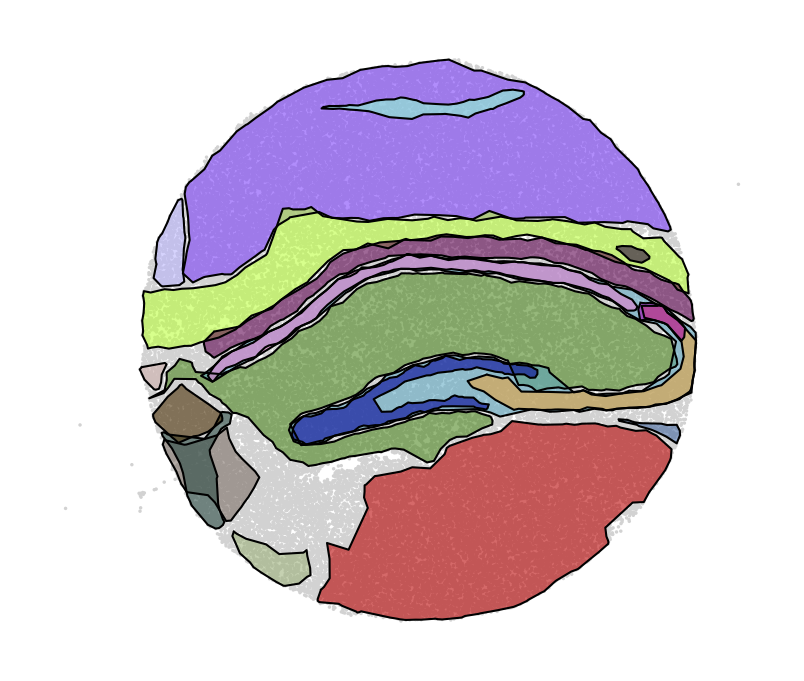
By computing boundaries (parameter alpha_max controls how tightly the boundary follows the spots. Increasing the value gives a boundary with greater curvature.)
nest.compute_multi_boundaries(adata, alpha_max=0.005, alpha_min=0.00001) nest.plot.multi_hotspots(adata)
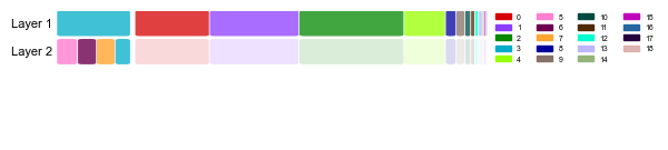
Nested structure plot allows for visualization of the nested hierarchical structure in the dataset, showing the existence of two layers (of overlapping hotspots) in the hippocampal formation, and one layer everywhere else in the dataset.
nest.plot.nested_structure_plot(adata, figsize=(5, 1.5), fontsize=8, legend_ncol=4, alpha_high=0.75, alpha_low=0.15, legend_kwargs={'loc':"upper left", 'bbox_to_anchor':(1, 1.03)})
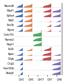
NeST is by design highly explainable as all coexpression hotspots derive directly from an ensemble of genes. We can confirm that the identified hotspots are meaningful by looking at these markers for the five coexpression hotspots representing the hippocampal formation.
markers = nest.geometric_markers(adata, [3, 5, 7, 8, 15])
markers_sub = {k: v[:3] for k, v in res.items()}
fig, ax = nest.plot.tracks_plot(adata, markers_sub, width=2.5, track_height=0.1, fontsize=6, marked_genes=[])