
Guanjue Xiang, Yuchun Guo, David Bumcrot, Alla Sigova. at CAMP4 Therapeutics Corp., Cambridge, MA, USA
Combinatorial patterns of epigenetic features reflect transcriptional states. Existing normalization approaches may distort relationships between functionally correlated features by normalizing each feature independently. We present JMnorm, a novel approach that normalizes multiple epigenetic features simultaneously by leveraging information from correlated features. We show that JMnorm-normalized data preserve cross-feature correlations and combinatorial patterns of epigenetic features across cell types, improve cross-cell type gene expression prediction models, consistency between biological replicates, and detection of epigenetic changes upon perturbations. These findings suggest that JMnorm minimizes technical noise while preserving biologically relevant relationships between features.
Guanjue Xiang, Yuchun Guo, David Bumcrot, Alla Sigova, JMnorm: a novel joint multi-feature normalization method for integrative and comparative epigenomics, Nucleic Acids Research, 2023;, gkad1146, doi: https://doi.org/10.1093/nar/gkad1146
 An overview of the four key steps in the JMnorm normalization procedure. (A) Step 1: orthogonal transformation. The correlated components of various epigenetic signals are transformed into mutually independent high-dimensional PCA dimensions. Each colored block on the left represents the signal vector of all epigenetic features at the nref or ntar cCRE regions in reference or target sample, respectively. Colored blocks on the right denote corresponding transformed PCA epigenetic signal matrices for reference and target samples. The yellow box in the middle represents the PCA rotation matrix learned from the reference signal matrix. (B) Step 2: cCRE clustering. Reference cCRE clusters are generated based on the reference data in PCA space with the average signal reference matrix shown as a heatmap. Target cCREs are assigned to reference clusters according to the Euclidean distances between the signal vector of the target cCRE and the average signal vectors of reference clusters in the PCA space. Within each cluster, the number of cCREs, shown as colored blocks within the insert, may vary between the reference and target samples. (C) Step 3: within-cluster normalization. Target signal matrix is normalized against the reference matrix using within-cluster quantile normalization as shown for Cluster k. (D) Step4: reconstruction of the JMnorm-normalized target signal matrix in the original signal space. The yellow box in the middle indicates the transposed PCA rotation matrix learned in the first step (panel A).
R version 4.0.0 or later Packages: readr, pheatmap, dynamicTreeCut
# create conda environment for JMnorm with required dependencies
conda create -n jmnorm r r-readr r-dynamicTreeCut r-pheatmap

# activate the environment
conda activate jmnorm

# git clone the JMnorm GitHub repository
git clone https://github.com/camp4tx/JMnorm.git

# start R
# source the script in R
# source("/path_to_JMnorm_folder/bin/JMnorm_core/JMnorm.script.R")
- The input Target signal matrix and input Reference signal matrix should be formatted as N-by-(M+1) matrices, where N represents the number of cCREs, and M represents the number of chromatin features. The first column of each matrix contains the cCRE IDs. The signal values in orignal linear scale for each chromatin feature in the cCREs are saved in the 2~M columns. The first row each matrix contains the cCREids and the chromatin feature name of each column.
- Example input Target / Reference signal matrices can be found in these links Target signal matrix & Reference signal matrix.
# Input reference signal matrix
>>> head ref.raw_sigmat.txt
cCREids	ATAC	H3K27ac	H3K27me3	H3K36me3	H3K4me1	H3K4me3	H3K9me3
1	0.927	0	0	0	0	0	0
2	0.235	0.17	0.023	0.611	0.014	0.062	0.038
3	1.684	2.701	1.453	0.741	0.819	1.376	5.44
4	0.829	1.017	0.627	0.413	0.455	0.455	2.712
5	2.385	1.427	1.292	0.602	1.159	3.49	6.337
6	3.79	0.732	0.636	0.293	2.049	1.057	0.244
7	2.793	0.681	0.406	0.219	1.085	0.954	0.27
8	3.204	0	0	0	0	0.309	0.098
9	1.264	0	0	0	0	0	0.134
10	1.364	0	0	0	0	0.315	0.062

# Input target signal matrix
>>> head TCD8.raw_sigmat.txt
cCREids	ATAC	H3K27ac	H3K27me3	H3K36me3	H3K4me1	H3K4me3	H3K9me3
1	0	0	0	0	0	0	0
2	0	0.104478	0	0	0	0.139552	0
3	0.385093	2.3354	0	0	0	2.47516	6.02857
4	1.41256	0.571749	0	0	0	0	2.91614
5	2.92286	1.86457	0	0	0	0	9.50857
6	1.82927	1.53252	0.855691	0	0	1.21057	0.347561
7	0	0.613636	0.510331	0	0	0.636364	0
8	0.394737	0	0	0	0	0	0
9	0.657895	0	0	0	0	0	0
10	0	0	0	0	0	0	0

# The chromatin features used in this example file: ATAC, H3K27ac, H3K27me3, H3K36me3, H3K4me1, H3K4me3, H3K9me3
Detailed instructions on using JMnorm can be found in the Getting started with JMnorm R markdown file. The testing signal matrices can be found in this link: https://github.com/camp4tx/JMnorm/tree/main/test_data
- The output target signal matrix after JMnorm should be formatted as N-by-(M+1) matrices, where N represents the number of cCREs, and M represents the number of chromatin features. The first column of each matrix contains the cCRE IDs. The signal values in orignal linear scale for each chromatin feature in the cCREs are saved in the 2~M columns.
- Example output target signal matrix after JMnorm can be found in this Target.JMnorm_sigmat.txt.
>>> head TCD8.JMnorm_sigmat.txt
cCREids	ATAC	H3K27ac	H3K27me3	H3K36me3	H3K4me1	H3K4me3	H3K9me3
1	0.068	0.05	0.099	0.025	0.002	-0.064	0.137
2	0.129	0.105	0.156	0.073	0.094	0.131	0.187
3	0.341	2.493	0.269	0.006	0.435	0.984	4.906
4	1.15	0.499	0.664	0.216	0.417	0.161	2.134
5	1.566	2.022	0.383	-0.018	0.408	-0.015	7.836
6	0.674	1.123	1.054	0.323	0.513	0.59	0.466
7	0.334	0.535	0.709	0.219	0.414	0.458	0.332
8	0.444	0.099	0.161	0.059	0.091	-0.048	0.208
9	0.604	0.104	0.162	0.05	0.096	-0.059	0.214
10	0.075	0.079	0.13	0.065	0.086	-0.101	0.179
- Since JMnorm normalizes epigenetic data by leveraging information from functionally correlated epigenetic features, we anticipate that simultaneous normalization of highly correlated features can yield better improvements with JMnorm. To help users more effectively select features with better correlations for JMnorm analyses, we computed pairwise cross-feature correlations for 538 epigenetic features in K562 cells using data from the ENCODE Consortium. Considering the substantial size of the output correlation matrix and the difficulties with visualization, we also set up a ShinyApp visualization tool for convenient and interactive exploration of the correlation matrix.
# 1, Open RStudio: Launch RStudio (Information about RStudio installation: https://rstudio-education.github.io/hopr/starting.html) on your computer.
# 2, Access the R script: Locate and open the R script named shinyApp.show.ENCODE.heatmap.R which is situated in the JMnorm/bin/ directory.
# 3, Modify the File Path: Inside this script, you need to adjust the file path to the data file you want to use. Change the existing path to point to the K562.raw_sigmat.mk.cor.txt file located in the JMnorm/test_data/ directory.
# 4, Execute the Script: After modifying the file path, you can run the script in RStudio. You can do this by clicking on the "Run" button, or by using the shortcut key (usually Ctrl+Enter or Cmd+Return).
# By following these steps, the script should launch a interactive ShinyApp paper, and you should be able to selecting a subset of epigenetic features and view their K562 correlation heatmap. If you run into any issues, ensure that the file paths are correct and that the necessary data files are present in the specified directories.
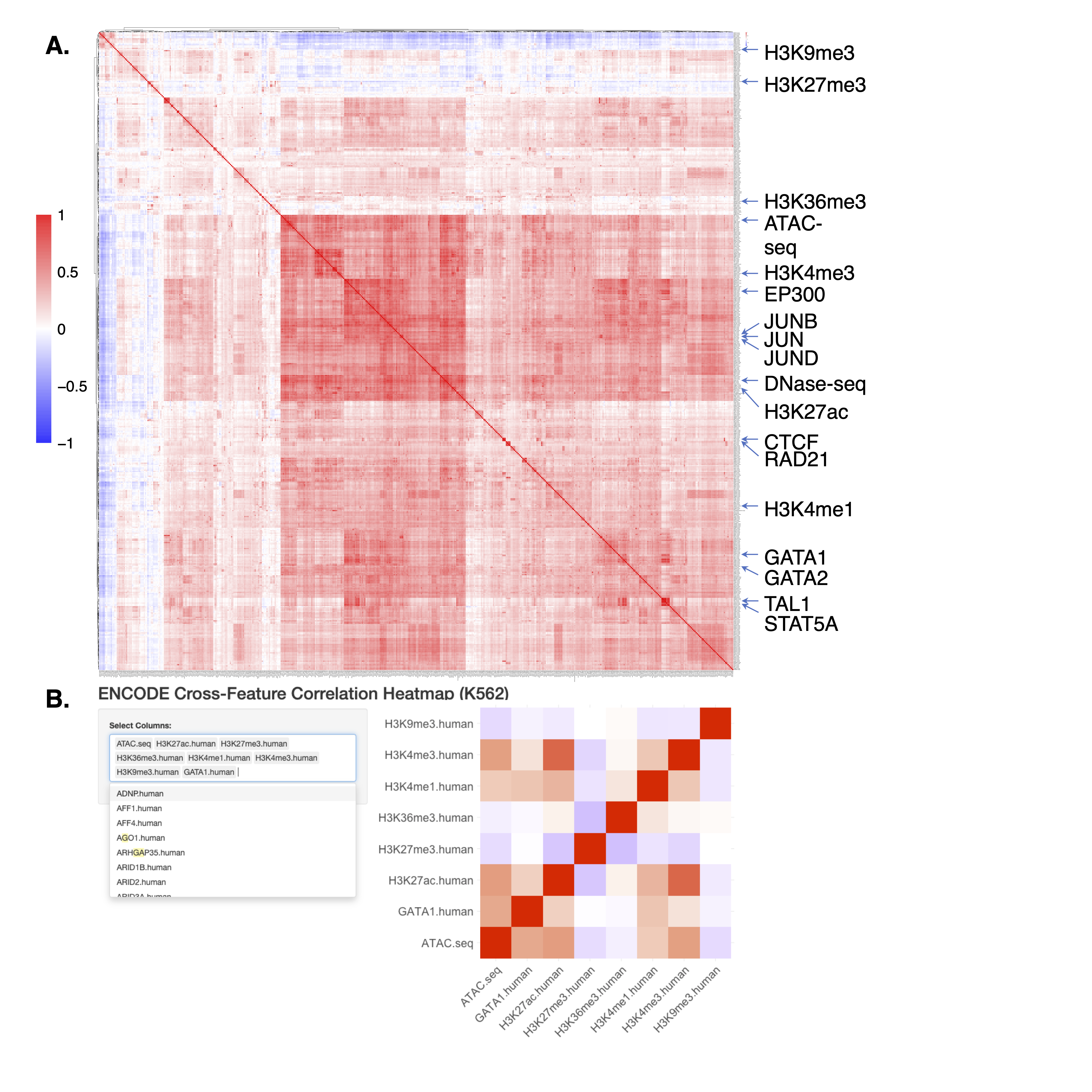 (A) The Pearson correlation matrix of 538 epigenetic features in K562 cells. (B) The ShinyApp visualization tool designed to aid in searching and visualization of a subset of features from the afore-mentioned correlation matrix.
For questions or issues, please either create an issue on the GitHub repository or feel free to reach out via the following email addresses: gxiang@camp4tx.com
This project is licensed under the GNU GENERAL PUBLIC License (Version >=2.0). See the LICENSE file for details.