Gaussian Infer

This is a proof of concept implementation for a small probabilistic programming language with a first-class exact conditioning operator. It is accompanying material to our paper "Compositional Semantics for Probabilistic Programs with Exact Conditioning".

Our implementation provides a type for Gaussian random variables, which can be combined affine-linearly, that is they can be added and scaled but not multiplied. Random variables can be conditioned on equality on numbers or other random variables. For example, creating two standard normal variables and setting them equal

x = N(0,1)
y = N(0,1)
x =.= y

is equivalent to conditioning

x = N(0,1/2)
y = x

This setup is sufficient to concisely express Gaussian process regression or Kálmán filters.

We provide two implementations, one using Python+numpy, the other one using F#+MathNet.Numerics.

Initial example: Gaussian regression

g = Infer() # instantiate inference engine

# some regression data
xs = [1.0, 2.0, 2.25, 5.0, 10.0]
ys = [-3.5, -6.4, -4.0, -8.1, -11.0]

plt.plot(xs,ys,'ro')

# make Gaussian random variables (prior) for slope and y-intercept
a = g.N(0,10)
b = g.N(0,10)
f = lambda x: a*x + b

# condition on the observations
for (x,y) in zip(xs,ys):
    g.condition(f(x), y + g.N(0,0.1))

# predicted means
ypred = [ g.mean(f(x)) for x in xs ]
plt.plot(xs,ypred)

plt.show()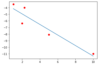

A DSL for Gaussians

We have added a decorator gauss which constructs a Gauss morphism from a function using a specialized form of normalization-by-evaluation.

# Denotes a morphism 1 -> 2
@gauss
def ex(x):
    y = x + 5*normal()
    return y, x

Structure

As F# is statically typed, we can inspect the relevant type signatures of the implementation. The core ingredient is an abstract type rv of Gaussian random variables, which can be combined linearly

type rv = 
    static member ( + ) : rv * rv -> rv       // sum of random variables
    static member ( * ) : float * rv -> rv    // scaling only with constants
    static member ( * ) : rv * float -> rv    // symmetrical ...
    static member FromConstant : float -> rv  // numbers as constant random variables
    (...)

The inference engine maintains a prior over all random variables. New variables can be allocated using the Normal method, and variables can be conditioned on equality using the Condition method.

type Infer =
    member Normal : float * float -> rv    // fresh normal variable with specified mean and variance
    member Condition : rv * rv -> unit     // condition on equality
    member Marginals : rv list -> Gaussian // marginals of a list of variable
    member Mean : rv -> float              // mean of an rv
    (...)

The typed version of the Gaussian regression example reads

open FSharp.Charting
open Infer

let make_infer() = 
    let infer = Infer()
    infer, infer.Normal, fun v w -> infer.Condition(v,w) 

let bayesian_regression_example() = 
    let infer, normal, (=.=) = make_infer()

    let xs = [1.0; 2.0; 2.25; 5.0; 10.0]
    let ys = [-3.5; -6.4; -4.0; -8.1; -11.0]

    let a = normal(0.0, 1.0)
    let b = normal(0.0, 1.0)
    let f x = a*x + b

    for (x, y) in List.zip xs ys do
      f(x) =.= y + normal(0.0, 0.1)

    let points = Chart.Point (List.zip xs ys)
    let regression_line = Chart.Line [ for x in xs -> (x, infer.Mean(f(x))) ]

    Chart.Combine [points; regression_line] |> Chart.Show 

Implementation

Some comments on the implementation and differences between the two versions.

The Python implementation features a class Gauss which represents an affine-linear map with Gaussian noise. This is precisely a morphism in the category Gauss described by [Fritz'20], and functions like then and tensor are provided to allow composition of Gaussian maps like in a symmetric monoidal category. All formulas directly match the paper. The class Infer represents the inference engine. The F# implementation, apart from being statically typed, is more minimalistic: We do not model full Gaussian maps but only the distribution part which is required for performing inference.

Numerics

In practice, in order to condition Gaussian variables one may compute a Cholesky decomposition of the covariance matrix (e.g. (2.25)). This is efficient and works well if the covariance matrix in question is positive definite (regular); one may also make observations slightly noisy, which corresponds to adding a small diagonal perturbation to the covariance matrix, making it positive definite.

We don't do this here, as our paper is precisely interested in the positive semi-definite case. Consider the linear regression example from before, then the noiseless observations

f(0) =.= 0.0
f(1) =.= 1.0
f(2) =.= 1.0

cannot be satisfied by any linear function f, hence inference should fail (this can be derived algebraically using the paper). In our implementation, we employ SVD and an explicit formula using the Moore-Penrose pseudoinverse for conditioning, and try to check the support conditions manually.

Nonetheless, the support condition is highly susceptible to rounding errors: Small perturbations will make the covariance matrix regular. This indicates the importance of an algebraic treatment like in our paper.

Further Examples

Kálmán filter

We show a 1-dimensional Kálmán filter for predicting the movement of some object, say a plane, from noisy measurements.

g = Infer()

xs = [ 1.0, 3.4, 2.7, 3.2, 5.8, 14.0, 18.0, 11.7, 19.5, 19.2]

# Initialize positions and velocities
N = len(xs)
x, v = [0] * N, [0] * N
x[0] = xs[0] + g.N(0,1)
v[0] = 1.0 + g.N(0,10)

for i in range(1,N):
    # Predict movement 
    x[i] = x[i-1] + v[i-1]
    v[i] = v[i-1] + g.N(0,0.75) # Random change to velocity 
    
    # Make noisy observations
    g.condition(x[i] + g.N(0,1),xs[i])

plt.plot(xs,'ro')
plt.plot([ g.mean(x[i]) for i in range(len(xs)) ],'g')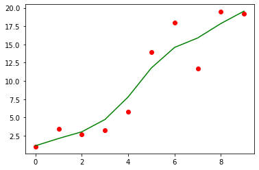

This is easily adapted to a 2-dimensional version, and changes to accelerations etc.

Gaussian Process Regression (Kriging)

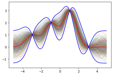
We showcase Gaussian process regression using the rbf kernel:

# rbf kernel
rbf = lambda x,y: 0.2 * np.exp(-(x-y)**2)

def gp(xs, kernel):
    K = [[ kernel(x1,x2) for x1 in xs] for x2 in xs ]
    return G.N(np.array(K))

# build GP prior
xs = np.linspace(-5, 5, 100)
ys = g.from_dist(gp(xs, rbf))

# condition exactly on observed datapoints
observations = [(20,1.0), (40, 2.0), (60, 3.0), (80, 0.0)]
for (i,yobs) in observations:
    g.condition(ys[i],yobs)

# plot sample functions
posterior = g.marginals(*ys)
for i in range(750):
    samples = posterior.sample()
    plt.plot(xs,samples,alpha=0.05)
    
# Plot means
means = np.array([ g.mean(y) for y in ys ])
plt.plot(xs, means, 'red')

# Standard deviation ± 3sigma
stds = np.array([ np.sqrt(np.abs(g.variance(y))) for y in ys ])
plt.plot(xs, means + 3*stds, 'blue', xs, means - 3*stds, 'blue')