Detecting Anomalies in the S&P 500 index using Tensorflow 2 Keras API with LSTM Autoencoder model.
- Machine Learning / Deep Learning
- Time Series Analysis
- Anamoly Detection
- LSTM
- Autoencoder
- python
- sklearn
- pandas, jupyter
- matplotlib, plotly
- tensorflow - keras api
It is a statistical technique that deals with time series data, or trend analysis. Time series data means that data is in a series of particular time periods or intervals. Data points may have an internal structure (autocorrelation, trend or seasonality). Time Series Analysis is used for many applications such as :
- Economic Forecasting
- Sales Forecasting
- Budgetary Analysis
- Stock Market Analysis
- Yield Projections
- Process and Quality Control
- Inventory Studies
- Workload Projections
- Utility Studies
- Census Analysis
Anomaly detection is about identifying outliers in a time series data using mathematical models, correlating it with various influencing factors and delivering insights to business decision makers. Using anomaly detection across multiple variables and correlating it among them has significant benefits for any business.
Read this article to understand more on how anomaly detection can help buinesses.
-
What are Autoencoders ? - An autoencoder is a neural network model that seeks to learn a compressed representation of an input. They are a self-supervised learning method that attempts to recreate the input.
-
LSTM - Recurrent Neural Networks, such as the LSTM, are specifically designed to support sequences of input data. They are capable of learning the complex dynamics within the temporal ordering of input sequences as well as use an internal memory to remember or use information across long input sequences.
-
Encoder-Decoder - The LSTM network can be organized into an architecture called the Encoder-Decoder LSTM that allows the model to be used to both support variable length input sequences and to predict or output variable length output sequences. In this architecture, an encoder LSTM model reads the input sequence step-by-step. After reading in the entire input sequence, the hidden state or output of this model represents an internal learned representation of the entire input sequence as a fixed-length vector. This vector is then provided as an input to the decoder model that interprets it as each step in the output sequence is generated.
-
LSTM Autoencoder - For a given dataset of sequences, an encoder-decoder LSTM is configured to read the input sequence, encode it, decode it, and recreate it. The performance of the model is evaluated based on the model’s ability to recreate the input sequence. Once the model achieves a desired level of performance recreating the sequence, the decoder part of the model may be removed, leaving just the encoder model. This model can then be used to encode input sequences to a fixed-length vector.
Import important libraries like pandas, numpy, matplotlib, plotly, tensorflow and sklearn.
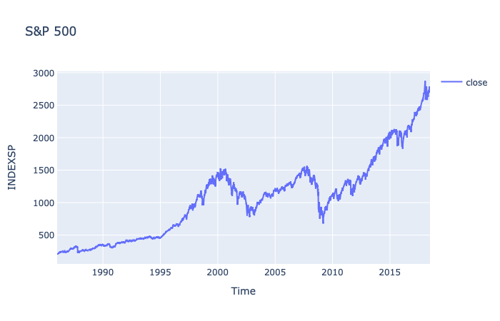
- Range: 1986->2018
- Frequency: 'D'- Mon->Fri
Split the dataset into 80% for the training set and remaining 20% for the test set.
The LSTM network takes the input in the form of subsequences of equal intervals of input shape (n_sample,n_timesteps,features).
Model Summary :
| Layer(type) | Output Shape | # Param |
|---|---|---|
| lstm (LSTM) | (None, 128) | 66560 |
| dropout (Dropout) | (None, 128) | 0 |
| repeat_vector (RepeatVector) | (None, 30, 128) | 0 |
| lstm_1 (LSTM) | (None, 30, 128) | 131584 |
| dropout_1 (Dropout) | (None, 30, 128) | 0 |
| time_distributed (TimeDistributed) | (None, 30, 1) | 129 |
Total params: 198,273
Trainable params: 198,273
Non-trainable params: 0
The metrics are saved inside the model variable, we can plot the training and validation loss wrt number of Epochs.
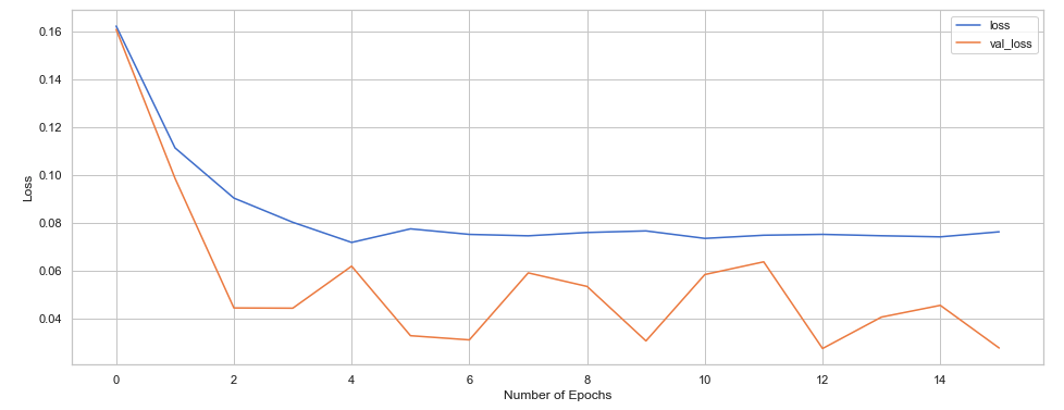
We have underfit the model as our val_loss<loss, we can change the parameters for a better fit.
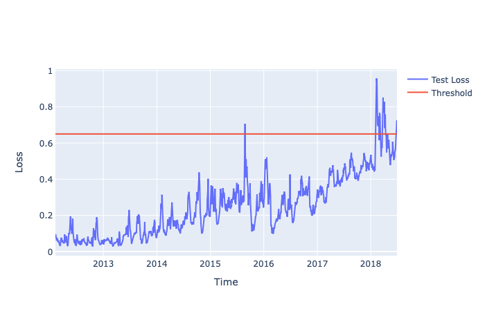
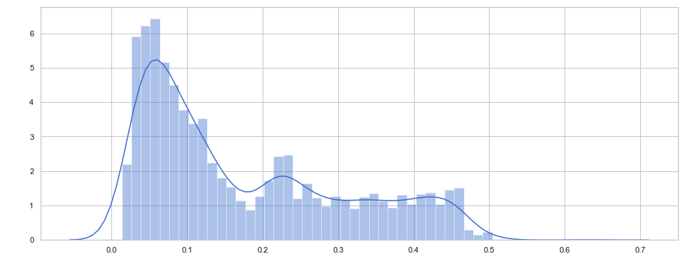 With the help of the distribution plot of the training loss, we can observe that very few observations have an error > 0.65. If we set threshold = 0.65, any error > 0.65 on the test loss will be considered as an anomaly.
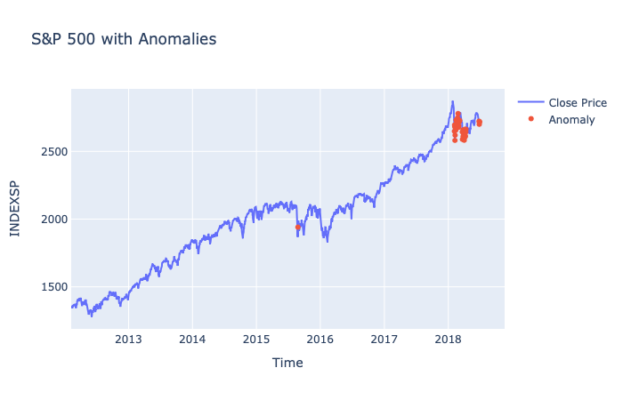
Plotting our threshold line at 0.65, all the loss values above it are anomalies
Depicting the anomalies with 🔴