This repository contains source code for the paper “Swiss Bank Savings versus Piggy Bank Savings: The Effect of Offshore Wealth on Estimates of Inequality and the Marginal Propensity to Consume”. The paper was authored by (alphabetically): Nicolas Charlton, Georgi Demirev (maintains this repo), Daniel Ruiz Palomo, Christoph Semken (maintains this repo), Joël Terschuur.
The first part of the README gives an executive summary of the paper. The second part gives short instructions on reproducing the results.
Survey data containing wealth estimates at the household level is often used in conjunction with heterogeneous agent models to study the impact wealth inequality can have on an economy, including through the marginal propensity to consume (MPC). Unfortunately, these data often suffer from under-representation and differential non-response from wealthy households near the top of the distribution, leading to biased wealth distribution estimates. Using offshore wealth data from Alstadsæter, Johannesen, and Zucman (2018), we propose a novel method for mitigating these issues and apply our methodology to the ECB's Household Finance and Consumption Survey (HFCS). We re-calibrate a consumption-savings model proposed by Carroll, Slacalek, and Tokuoka (2014) using wealth distributions estimated with and without offshore. We find that correcting for offshore wealth leads to important changes in the predicted average MPC and distribution of MPCs for several countries.
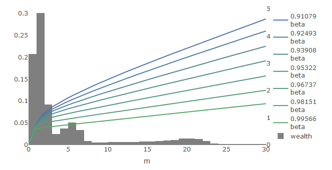
To add estimates of offshore wealth to household liquid assets from HFCS we fit a Pareto Model to the top decile (by wealth) of households. This way we estimate the individual share of offshore wealth for each household in the survey (for each country). To estimate the marginal propensity to consume we implement a version of the Carroll, Slacalek, and Tokuoka (2014) model, which is in turn based in part on earlier work by Krussel and Smith (1998). The model is characterized by heterogeneous agents (in preferences) and idiosyncratic income shocks (both permanent and transitory). We calibrate the model by choosing parameters (in this case the discount factors of different agent types) such that the wealth distribution resulting from simulating the economy is close to the wealth distribution observed in the data. This parameter tuning is done with a genetic algorithm.
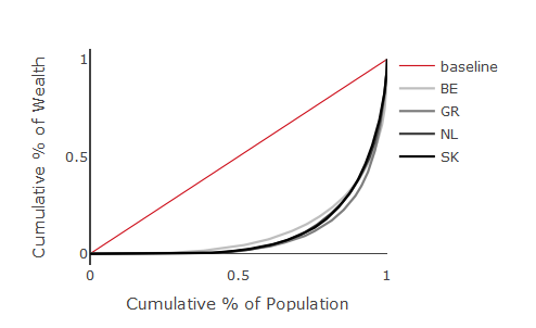
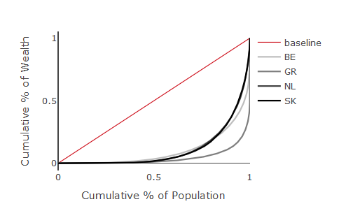
By adding offshore wealth to liquid assets in the HFCS we find a noticeable increase in the GINI measure of inequality for all countries. The magnitude of the change is about 0.02 - 0.03 for most countries (with Greece showing the highest change of 0.11 and Netherlands the smallest with 0.002).
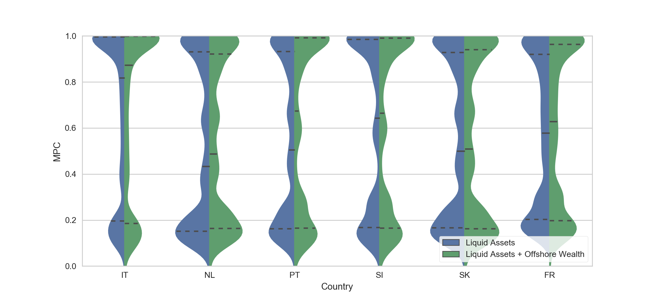
We find that after adding offshore wealth the estimates for the MPC change by between 0.03 and 0.09 for most countries - a change with a meaningful economic significance.
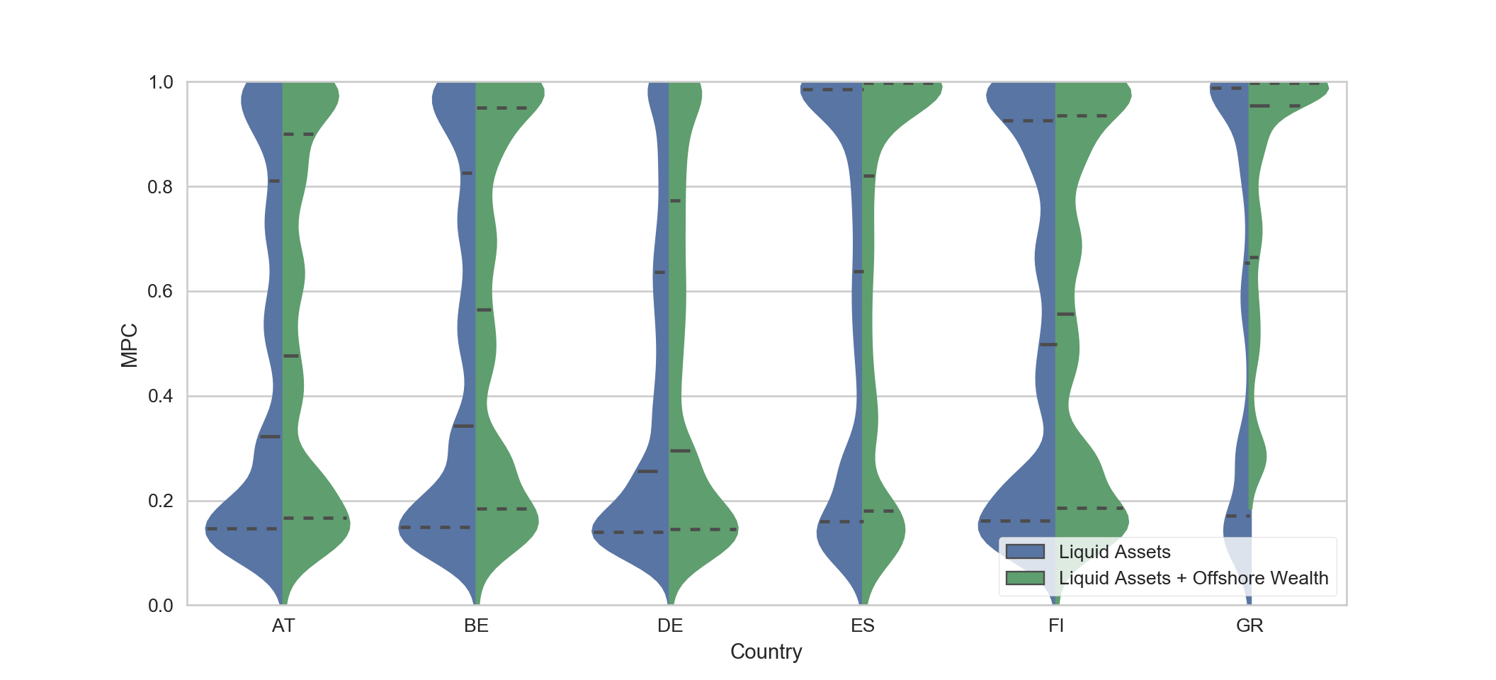
Furthermore we find a strong correspondence between the GINI of the target wealth distribution used for calibrating the model and the implied marginal propensity to consume:
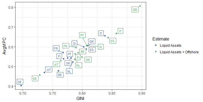
For a detailed exposition of our methodology and findings please refer to the full text of the paper.
- R/ - R source code
- R/00_libraries.R - needed packages
- R/01_gini_summaries.R - interactive generation of data summaries (HFCS + offshore)
- R/02_generate_targets.R - generates the wealth deciles used as targets in the calibration
- R/03_calibration.R - runs the calibration (with a country parameter)
- R/04_mpc_analysis.R - solves final models and produces summaries of the results
- R/classes/ - R6 classes used for the model
- R/classes/krussell_smith.R - implements a version of the Krussel-Smith Economy. Also includes an agent class.
- R/classes/shocks_util_prod.R - various classes for utility functions, production functions and shock generators.
- R/functions/
- R/functions/calibration.R - functions for calibrating the model
- R/functions/descriptives.R - functions for data exploration (also for adding offshore wealth)
- R/functions/dynprog.R - functions regarding dynamic programming (i.e. policy function iteration)
- R/functions/utils.R - misc helpers (reading data, averaging across imputations of the HFCS etc)
- data/
- data/generated/ - Rdata files generated for or by calibrations. Can be loaded into an R environment
- data/generated/decile_targets.RData - used for calibration
- data/generated/final_models.RData - final solved model objects
- data/generated/ginis_liq.RData - GINI indices
- data/generated/quintile_targets.RData - alternative targets (not used)
- data/HFCS_UDB_1_3_ASCII/ - input data containing the HFCS. Not included in the repo due to confidentiality. Available upon request from the ECB.
- data/generated/ - Rdata files generated for or by calibrations. Can be loaded into an R environment
- deliverables/ - pre-compiled HTML files summarizing key results
- R 3.5
- RStudio 1.1 (recommended)
- R packages listed in R/00_libraries.R
- Python 3.5
- Python package seaborn (only for MPC violin plot)
To estimate wealth distributions using HFCS data, access to the data needs to be requested from the ECB. Once authorization has been granted, the text-only source files should be placed in data/HFCS_UDB_1_3_ASCII/.
The folder should then contain the files listed below (MD5 hash sums included):
- D1.csv 1156368390ce53c99fb4ec6011b7167f
- D2.csv 1c6b837bf5434f848c095f213d8dd322
- D3.csv f8505023a1232e610b77fbf5d562babb
- D4.csv 3d2fd9c5901096ec2ff09275552fcb14
- D5.csv 76fcbd6fe0083940d4fa0427454bb900
- H1.csv 595f8514ed5a321f4df02c6ed18ea392
- H2.csv 2ed9f16db3bc60c1f75310e7f364fd89
- H3.csv 8bd17ce2c572b661fc19a51b79f1c9ee
- H4.csv d4d77f4f9350b947102299c746bbdeed
- H5.csv 63c2ebffdc53f3ffaff05a99838df476
- P1.csv e11fa0133a516e018bffbea08d329566
- P2.csv cec57e8bc4bfc2d9523fc2fdb413786c
- P3.csv a5223b91668a9f9cfd5794685ad8b9fc
- P4.csv 7737c5e67cd4d555ce37db2c9ae0f586
- P5.csv d0c8c00ed9af2a875774b4bcd4a1442e
- W.csv 85c72275ea6479e83119a1af5babd19a
To create summary statistics about wealth distributions estimated from the HFCS data, with and without the offshore adjustment, knit data_summary.Rmd. Alternatively you can interactively analyze the data using R/01_gini_summaries.R
To calibrate the model, you first need the empirical targets. These are created by R/02_generate_targets.R (and also exist as an RData file). Next change the parameters in and run R/03_calibration.R. The country of interest (2 digit country code), target wealth distribution and input values can be changed at the beginning of the file. A folder called calibration_checkpoints/ should be created in the root directory to allow for progress to be saved.
The output of each calibration run consists of a .csv file with the tested parameters, wealth deciles and loss compared to the empirical targets, and a .txt file containing log messages. The files were aggregated and best fit was chosen in a spreadsheet program. Unfortunately this means that this part is not fully reproducible.
The summary of the calibrated models used in the paper can be created without having to re-calibrate the model by knitting mpc_results.Rmd. The values for the Ginis and the solved models will be loaded from ginis.RData and final_models.RData (both inside data/generated/), respectively.
Alternatively you can explore the results interactively using R/04_mpc_analysis.R