The basic problem of this exercise is to create a model capable of predicting the arrival delay time of a commercial flight, given a set of parameters known at time of take-off.
To feed the application we will use data published by the US Department of Transportation: http://stat-computing.org/dataexpo/2009/the-data.html
In order to have a better understanding of the data and have a spatial vision of the quantitative variables we have performed a principal component analysis where we can observe from a better perspective which attributes are correlated.
In this analysis we removed non quantitative variables as are not relevant for the analysis, this variables are: unique carrier code, plane tail number, origin IATA airport code, destination IATA airport code, reason for cancellation.
In the following table we can see the percentage of variance in each principal component, we can conclude that the first three PC are the ones who will contain the bigger amount of the information.
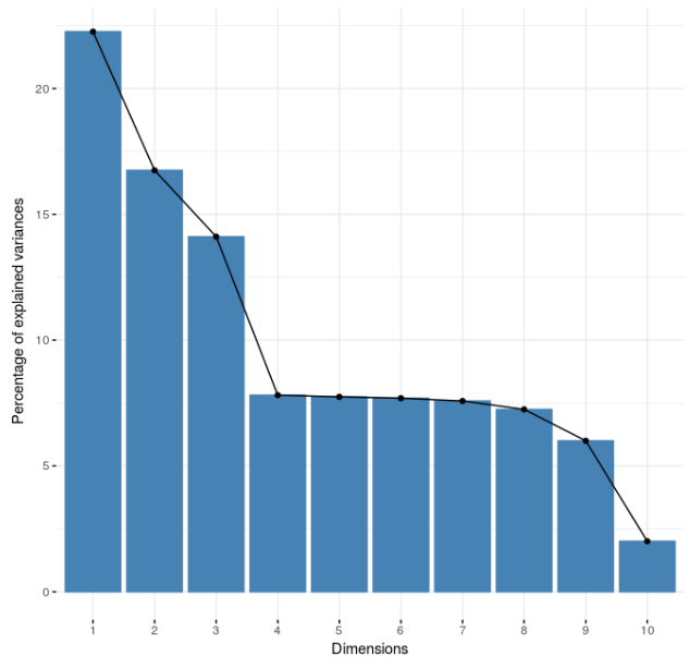
Scree plot
If we take a look at the first component we realize that the arrival delay is correlated with the actual departure time, scheduled departure time, scheduled arrival time and departure delay.
To get a better view of the relation of the variables we plot the level of correlation of the variables from the two main principal components, the PC1 is the most relevant for our analysis.
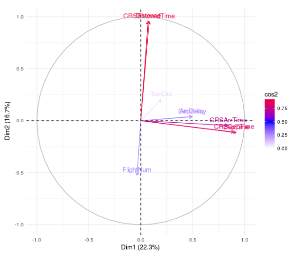
PCA variables
The analysis shows us that the departure delay (DepDelay) and the actual arrival time (ArrDelay) variables are highly correlated, if we take a look at the level of linear dependence between them we get a value of 0.93150, which is really high.
If we plot the linear relationship we can clearly appreciate the correlation in a sample of the data set:
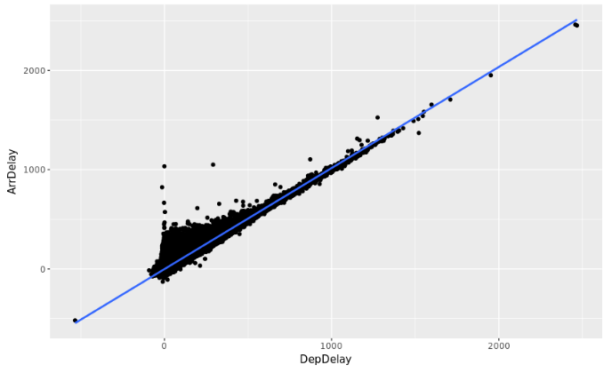
Scatter Plot
So this problem can be solved using a regression model, in this case linear regression, to predict the value of the arrival time.
As we see in the analysis we don’t need all the variables for the creation of the model, only few of them will be needed, but first we will remove from the data set those who are forbidden:
- ArrTime
- ActualElapsedTime
- AirTime
- TaxiIn
- Diverted
- CarrierDelay
- WeatherDelay
- NASDelay
- SecurityDelay
- LateAircraftDelay
Once we remove forbidden variables now we will remove those unnecessary and non quantitative ones:
- TailNum
- UniqueCarrier
- Cancelled
- CancellationCode
The last step consist in type casting remaining variables:
col("Year").cast(IntegerType),
col("Month").cast(IntegerType),
col("DayofMonth").cast(IntegerType),
col("DayOfWeek").cast(IntegerType),
col("DepTime").cast(IntegerType),
col("CRSDepTime").cast(IntegerType),
col("CRSArrTime").cast(IntegerType),
col("FlightNum").cast(IntegerType),
col("CRSElapsedTime").cast(IntegerType),
col("ArrDelay").cast(IntegerType),
col("DepDelay").cast(IntegerType),
col("Origin").cast(StringType),
col("Dest").cast(StringType),
col("Distance").cast(IntegerType),
col("TaxiOut").cast(IntegerType)
We only choose the most relevant ones before passing the features to the linear regression model, in order to compute only the necessary attributes and after test the rest of them are not useful for the model creation we deduce the following variables are the most relevant for the creation of the model:
new VectorSlicer()
      .setInputCol("rawFeatures")
      .setOutputCol("features")
      .setNames(Array("DayOfWeek", "DepTime", "CRSDepTime", "CRSArrTime", "CRSElapsedTime", "DepDelay", "OriginIndex", "DestIndex", "Distance", "TaxiOut"))
The main one will be the departure delay as we see in the correlation analysis, the day of the week stands out over the rest of the date variables, all related with times are important and origin and destination could be relevant as well.
As we have variables highly correlated and the outcome can be an infinite number of possible values we found linear regression a model that could fit well.
new LinearRegression()
    .setLabelCol("ArrDelay")
    .setFeaturesCol("features")
    .setMaxIter(10)
    .setRegParam(0.3) // Increasing lambda results in less overfitting but also greater bias
    .setElasticNetParam(0.8) // Reduce overfitting
We set 0.3 as the regularization parameter, increasing lambda results in less overfitting but also greater bias. To reduce the possible overfitting ElasticNet mixing parameter will take a value of 0.8.
To validate the model we are going to perform a cross validation technique to evaluate the predictive model we got in the last step.
The validation consist in partitioning the original dataset into a training set to train the model, and a test set to evaluate it. In our case we decide to partition the dataset into 4 subsamples as we are using k-fold cross-validation.
new CrossValidator()
      .setEstimator(lrPipeline)
      .setEvaluator(evaluator)
      .setEstimatorParamMaps(paramGrid)
      .setNumFolds(4)
The result is very satisfactory, the model has an accuracy of almost 93% of success.
+--------------------+--------+------------------+
|            features|ArrDelay|        prediction|
+--------------------+--------+------------------+
|[2.0,2.0,2355.0,7...|      41|16.444628543191072|
|[2.0,3.0,2110.0,4...|     163| 163.9297539624578|
|[2.0,4.0,2110.0,2...|     162|166.36673117053616|
|[2.0,4.0,2355.0,5...|      13|2.2843791030856266|
|[2.0,5.0,2110.0,2...|     172|168.28347710130242|
|[2.0,5.0,2227.0,2...|      86| 89.82717055197509|
|[2.0,6.0,2350.0,8...|      12| 4.011101885311394|
|[2.0,13.0,2347.0,...|      11|  16.6427724100514|
|[2.0,13.0,2355.0,...|      22|  9.63024344266627|
|[2.0,13.0,2355.0,...|       8|10.772730840730997|
|[2.0,14.0,1950.0,...|     256|258.73194755034314|
|[2.0,14.0,2340.0,...|      35|24.899201199362768|
|[2.0,15.0,2328.0,...|      71| 45.63285356655041|
|[2.0,17.0,2340.0,...|      32|27.295218995360766|
|[2.0,18.0,2350.0,...|       3|14.702072796139891|
|[2.0,18.0,2359.0,...|       8|25.697157932718415|
|[2.0,20.0,2355.0,...|      13|14.048278962082218|
|[2.0,26.0,30.0,44...|      24|-3.656287511356065|
|[2.0,28.0,2359.0,...|      22|18.918287674859595|
|[2.0,29.0,2145.0,...|     162|154.35528107531368|
+--------------------+--------+------------------+
only showing top 20 rows

Accuracy: 0.9267017196272831
Run SBT run command passing as first argument the file to process:
user@host:/flight-delay-prediction$ sbt "run data/2007_sample.csv"Run SBT package command to generate .jar file:
user@host:/flight-delay-prediction$ sbt packageEnter to Hortonworks Data Platform sandbox, download the data file and put it into HDFS:
[root@sandbox ~]# hadoop fs -mkdir /tmp/data
[root@sandbox ~]# hadoop fs -put /tmp/data/2007.csv /tmp/data/
Copy project .jar file into the HDP sandbox and submit the spark yarn task:
[root@sandbox ~]# spark-submit --master yarn --class App flight-delay-prediction_2.11-0.1.jar /tmp/data/2007.csv