Creating the executable transformations from RegDNA logical transformations
We describe here the process of translating logical transformations written in RegDNA into an executable version following RegDNA’s model of computation. We use generators known as RegPots to create the executable version for a particular platform. In this case we will show how we generate artefacts in the executable language called Xcore to represent the executable version of the logical transformation rules.
We will show this with reference to full examples.
As prior reading we recommend that you read the RegDNA specification
The examples RegDNA files are stored in the src directory in an open-source GitHub repository here
The examples generated XCore files are stored in the src directory in an open-source GitHub repository here
The RegDNA specification outlines a model of computation that provides performance, maintainability, excellent lineage, and the ability to visualise the process of computation in concepts familiar to users of Excel.
The concepts are used also in modern analysis frameworks such as Apache Spark.
As described in the RegDNA spec (link), we see that platforms generated from RegDNA files will follow a model of computation, which can be easily visualized by users of Excel, and can be summarized as meeting the following properties:
- Immutable dataset to dataset transformations
- Immutable dataset to dataset transformations
- Operations that translate from attributes to a single attribute
- Immutable operations and transformations
- Side effect free operations and transformations
- Limits on complexity
Xcore makes use of Xtend (sometimes called XBase) which is a java like language, Xcore is often called ‘modeling for programmers and programming for modellers’ which highlighted it as a good initial choice for executable transformation rules, it also tightly related to Ecore.
Xcore is an object-oriented language, which can translate itself to Java.
The approach taken to generate XCore can be applied to other Object-oriented languages also like Python, Python Django, or C#, Java, or Java Spring. We note that the generation of the XCore classes is automated, but currently we do need to do some manual changes to the generated XCore to address what cannot be done automatically, or relate to idiosyncrasies of XCore, we document these and strive to make as few manual changes required as possible.
The generation process will create a class for each data set. We can consider the class as the template or ‘cookie cutter’ for the datasets.
Populated datasets will be described by objects (instances of the class) which have actual data. The dataset can be considered conceptually as a number of rows, each with the same structure, in a table. A class for the dataset will be named with _Table postfix.
The fields of the class will be types like int or string for items of the datasets related to the input layer, and will be operations (functions) on the slice or output layer or union dataset.
This diagram shows a subset of the datasets, populated. For conciseness it only shows a subset of attributes on a subset of input layers (specifically ones that provide data fto the F05.01 finrep report)
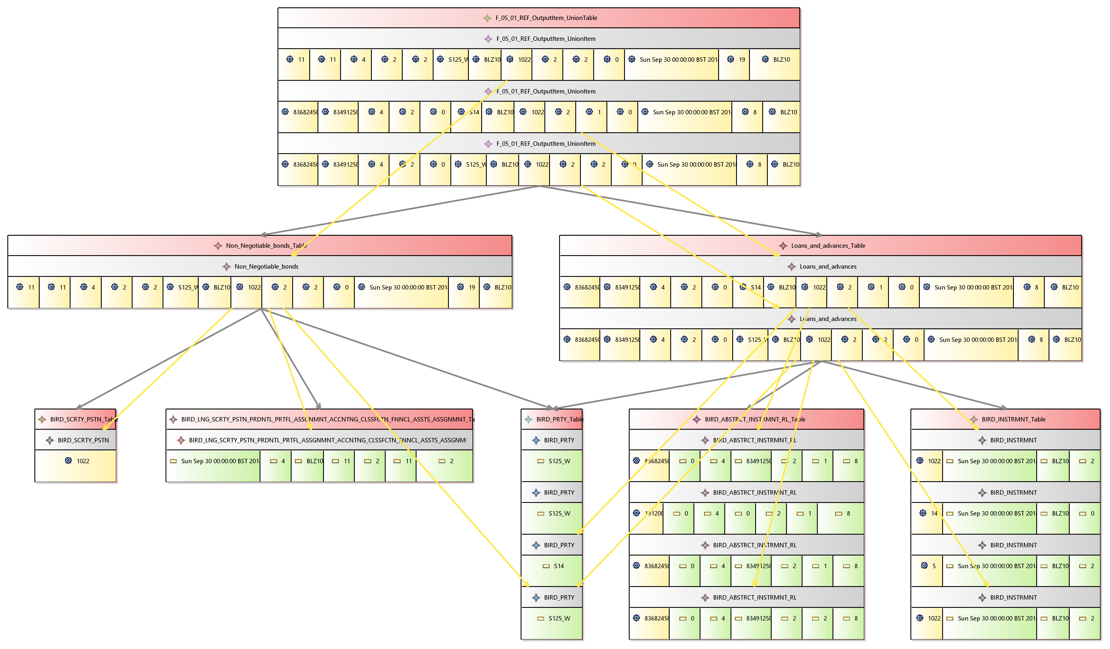
Note that inthis picture we havent shown the attribute names , which would make a bit clearer. The red boxes relate to datasets, which conatains a set of rows. The grey lines show dependant datasets. The grey boxes relates to rows which contain iether attributes or operations, the yellow lines show which rows are dependant upon which rows. The green boxes show attribute values, and the yellow boxes show operations (functions) which have been executed to provide a number. We describe this in more detail below.
In total we have a dataset for each entity in the input layer. We have a dataset for each slice, which is to be created by transforming some datasets in the input layer. We have a dataset per report which ’unions’ or ‘adds together’ the data sets for all slices in that report. We have a dataset for each output layer (so again one for each report template), and this is just a direct copy of the dataset which unioned the slices together. Once we have the output layer data set, we can apply the filters and aggregation from the reports In RegDNA.
We create one dataset per report cell, that report cell conceptually is a single table that has one row, which has one column, and the instance (object) of that class holds the value of that report cell.
We have classes that represent each data set. We describe here how we name the classes.
If the data set relates to an input layer entity then we call it <entity_name> _Table (e.g. BIRD_PRTY_Table, representing the table and will contain a list of objects with the a class <entity_name>_Table (e.g. BIRD_PRTY), The class <entity_name> (e.g. BIRD_PRTY) can be considered to represent a row , it has fields that can be considered as columns, these will have types such as String or int or a particular enumeration.
If the data set relates to an output layer then we call it <report_template>_output_item_Table (e.g. F05.01_REF_output_item_Table, representing the table and will contain a list of objects with the a class <report_template>_output_item (e.g. F_05_01_REF_Output_item ) . The class <report_template>_output_item can be considered to represent a row , it has fields that can be considered as columns, these will be represented as operations(member functions) on the class.
If the dataset represents a report cell it is named as Cell_<report_name>Output_item_row<row_name>col<column_name> for example Cell_F_05_01_REF_OutputItem_row_0010_col_0005
If the class represents a slice, then it has the name <slice_name>_Table E.g. Loans_and_advances_Table table and will contain a list of objects with the a class <slice_name> (e.g. Loans_and_advances) . The class <slice_name> can be considered to represent a row. Note that slices for report are always subtypes of an abstract class called < report_template>_OutputItem_Base, e.g. F_05_01_REF_OutputItem_Base. This helps us to union many slices together and enforces the slices to have the same structure (the same set of operations names)
If the class represents a unioned set of slices for a report, then it has the name <report_template>_OutputItem_Base e.g. F_05_01_REF_OutputItem_UnionTable.
Classes exist within packages, which group together a set of classes. The package and its classes are usually stored in a file with the same name as the package. Each class in a package must have a different name, but it is possible to have two classes with the same name if they are in the different packages. Slices, base classes, and unioned items related to a report will all be in a package named package <report_template>_OutputItem_Logic, e.g. package F_05_01_REF_OutputItem_Logic.
Let us take a look at an example XCore class representing an input layer entity as BIRD_PRTY_Table and the Xcore class representing the rows as BIRD_PRTY it is generated from the RegDNA file.


The key annotations (which start with @key) preserve some information from the original model, but do not affect executable behaviour.
We see that this is almost exactly the same as the RegDNA version of the model, because RegDNA uses a cutdown version of Xcore as its representation of data models. If we were to generate Python or C# then overall the files would look similar but use python and c# convention for describing classes.
Note that we are representing each attribute of the entity with a type like int , string, or and enum. The enumerations are described in another XCore file, which again is pretty much identical to the RegDNA file (given the similarity of Xcore and RegDNA) we provide a snippet here:

Note that these are Xcore classes that generate Java classes, Xcore itself can be run as an interpreted language, or the Java classes can be compiled and then run as pure Java with standard java debuggers, execution environments, etc.
We saw above that when representing attributes used in datasets to represent input layer entities that these have a type of int. double. String, or enumerated field. In Object-Oriented terminology we call these instance fields.
The contents of some other datasets (such as slices, unioned slices, and output layer entities, and report cells) are derived from these input layer datasets.
So the other datasets do not use instance fields to represent the attributes, but instead we use operations, which in Object Oriented terms we can call these member functions.
We show an example below for the Loans and Advances Slice:

We remind ourselves that this is generated from the generation rule for loans and advances as shown previously, hopeful you can see the resemblance where we have an operation for each of the per attribute transformations.

We always use the @dep annotation to highlight for each operation what are its dependent inputs, these are generated in the generation process. We use the dependency annotations a lot when finding the detailed lineage.
There are other ways to find lineage, such as parsing the abstract syntax tree of the function body, this would not be too difficult in XCore (the AST is very easy to access in Xcore), but it is much harder in other languages so we prefer to use the approach of dependency annotations, which are machine readable and can be used to build lineage visualisations.
Notice that an instance of this class ‘Loans_and_advances’ can be considered as a row in a dataset.
An important point here is that the single row has a link to single rows in dependant data sets. The row might link to one row from a dependant dataset or more than one (if it needs to net data from some rows for example).
So highlighted in yellow that we see here that we have a link to a row from BIRD_PRTY, (see refer BIRD_PRTY bIRD_PRTY ) and that to calculated the Institutional sector we on the Loans_and_advances row we reference an attribute (or operation) on the dependant row.
So how do those links to dependant rows get set? We describe this in the next section as operations that derive datasets (compared to the operations that derive attributes described in this section)
For data sets that are not from the input layer, we consider these as derived datasets.
So, for example the one for the slice Loans_and_advances with the class called Loans_and_advances_Table Here is the code.

Not again that this relates to the generation rule.
In the refers section it refers to the tables that are needed to get data from, these are the input tables mentioned in the generation rule. These relate to the source data sets. We may also have some more input tables here which are required to join those tables together, these relate to the full set of tables required for the
The operation, in this case calc_loans_and_advances (which follows the naming convention of calc_<slice_name>) is the technical implementation of filter, and the technical implementation of the hidden join.
We can see in the example the filter is encoded as an If statement , in this case we can see clearly that the filter of the generation rule and check that the TY_INSTRMNT is set to other_ loans, or credit_card_debt etc. In XCore we need to reference the enumerated literal name as upper case. Not the if we edit the XCore file we have autocomplete and validation features to help us.
Regarding the implementation of the ‘hidden join’ This calculation creates each of the rows for their slice in turn, and on the rows it sets precisely what are its dependant rows by setting the ‘refers to’ fields, which represent the association relationship to that rows dependant rows. So, we see we have dealt with dependant tables in this class, and create the dependencies between rows. Sowing the seed for excellent row lineage which when combined with operation dependencies enables cell lineage.
We should and will also set the dependencies of this function in @dep annotations, this then gives full transitive lineage and enables divisible lineage. This is an important step to give excellent lineage to show what it is truly required from the input layers to populate a single output layer, or even a single cell (pic to be provided)
So, we have described, hopefully clearly , how those refers fields got set in classes such as those for the rows of a slice. But in this class for the Table, how do we set the refers items so that they clearly point to populated datasets that it depends upon such as bIRD_PRTY_Table? How do we ensure that these datasets were already populated before we start getting rows from them and linking new rows to those rows that they are dependent upon? This is the responsibility of the init() function which we describe shortly.
The union just adds together the members of the slice. All slices for a report have a common superclass, so we can put them together in a list.

For the dataset for the report cell, we provide an example below

The init function calls the init function from the Orchestrator class, which is a component of the Desktop Regpot stored here
The orchestrator is responsible for creating the populated data sets as object instances (instances of the classes we discussed previously) and keeping a list of populated datasets.
The init function looks at the types of the referred to tables and makes a correct assumption that there should only be one populated dataset for each. It tries to find that populated dataset in the set of populated datasets, if it cannot find it then it creates it. If it cannot find a source dataset that represents an input layer entity then it will create it by loading in the XMI file with the same name, as we initially create XMI files with tools support for each of the input layer entities we will use (link to be provided to tutorial on making test data)
If it cannot find a source dataset, and the dataset is not related to an input layer table (perhaps it is related to a slice or derived table or union of slices) then it will create it by executing the init function for its related class, that starts a chain of processing which will call init on any datasets that it is dependent upon until it reaches dataset related to an input layer entity.
We note that a populated data set for a slice, will have its ‘refers’ attributes set. Note that the operations use those refers to attributes. Because we have classes that represent rows, it would be easy to mistakenly think that we call these operations and store the result as items in the rows (like cells in a row in Excel) , but this is not the case. We only call the functions when we need to (e.g. when we want to calculate a report cell)
As excel/CSV is ubiquitous, and is a great way to show populated datasets, we provide a means create a csv file for each populated dataset. The orchestrators’ main function will call all init functions as needed to set the ‘refers’ items of the classes, and then for each derived dataset it will call each operation to find out the rows created in data sets, and the values to put in cells.
[TODO]
[TODO]