bayes_dip

bayes_dip implements the Linearised Deep Image Prior, a framework for estimating uncertainty of DIP reconstructions.

The method and experiments on Computer Tomography data are described in the paper "Uncertainty Estimation for Computed Tomography with a Linearised Deep Image Prior" (arXiv). Outputs of our experiment runs are available from Zenodo.

Documentation of the library is available here.

The implementation uses the PyTorch framework.

Experiments

We use hydra for all experiment scripts. The configuration files are placed in experiments/hydra_cfg and provide default values. Values can be overridden and config groups can be selected from the command line; see hydra's docs for details. Each run of an experiment script run writes it's outputs to a new directory named after the current time; it also contains the configuration of the run in a sub-folder .hydra/. Python commands specified below should be executed from the working directory cd experiments, using an environment including the required packages (see Setup environment).

Walnut

As a preliminary, the walnut data needs to be placed in experiments/walnuts: Download Walnut1.zip and unzip to experiments/walnuts/Walnut1. The data is described in Der Sarkissian et al., "A Cone-Beam X-Ray CT Data Collection Designed for Machine Learning", Sci Data 6, 215 (2019); see also the containing Zenodo record and this code repository.

The sparse ray transform matrix for the fan-beam like 2D sub-geometry can be downloaded from here and needs to be placed in experiments/walnuts/single_slice_ray_trafo_matrix_walnut1_orbit2_ass20_css6.mat; alternatively, it can be created with examples/create_walnut_ray_trafo_matrix.py.

The reconstruction process with model uncertainty is split into the following steps (commands are exemplary):

1. Obtain an EDIP reconstruction

The output of this step can be downloaded from here, and extracted into experiments (resulting in experiments/multirun/...). This is the recommended way of obtaining the reconstruction, as the default configuration in experiments/hydra_cfg/experiment/walnut.yaml includes load_dip_params_from_path=multirun/2022-01-10/13-44-18/0/, i.e. the experiments by default try to load from this path.

Nevertheless, the EDIP reconstruction can be reproduced as follows. We initialize the DIP network with pretrained weights (obtained with this script as suggested in arXiv:2111.11926. Since the default configuration in experiments/hydra_cfg/experiment/walnut.yaml includes load_pretrained_dip_params=outputs/2021-12-02/17-23-12/params/model_walnut.pt, you can just unpack the above zip file into experiments (resulting in experiments/outputs/...) and run:

python dip.py experiment=walnut

to obtain an EDIP reconstruction. Of course, standard DIP reconstruction without pretraining is also possible by setting load_pretrained_dip_params=null, but we expect that a higher number of dip.optim.iterations is needed in this case.

2. Run Linearised DIP marginal likelihood optimisation

python dip_mll_optim.py experiment=walnut mll_optim.include_predcp=True mll_optim.predcp.scale=50.

This runs the hyperparameter optimisation for Linearised DIP (TV-MAP); in order to run Linearised DIP (MLL), specify mll_optim.include_predcp=False (instead of =True).

Let the output path of this step be $OUTPUT_LIN_DIP.

3. Generate samples from the predictive posterior

Estimating uncertainty now requires two final computations: assembling the covariance matrix in observation space ("cov_obs_mat") and drawing samples from the predictive posterior. These are performed by

python sample_based_density.py experiment=walnut use_double=True inference.load_path=$OUTPUT_LIN_DIP inference.cov_obs_mat.eps_mode=abs inference.cov_obs_mat.eps=0.1 inference.save_cov_obs_mat=True inference.save_samples=True inference.reweight_off_diagonal_entries=True inference.patch_size=1 inference.patch_idx_list=walnut_inner

Let the output path of this step be $OUTPUT_SAMPLES.

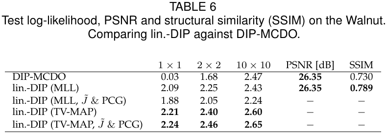
The samples are saved in the above run, allowing for efficient re-evaluation with e.g. a different inference.patch_size:

python sample_based_density.py experiment=walnut use_double=True inference.load_path=$OUTPUT_LIN_DIP inference.load_samples_from_path=$OUTPUT_SAMPLES inference.load_cov_obs_mat_from_path=$OUTPUT_SAMPLES inference.cov_obs_mat.eps_mode=abs inference.cov_obs_mat.eps=0.1 inference.save_cov_obs_mat=False inference.save_samples=False inference.reweight_off_diagonal_entries=True inference.patch_size=2 inference.patch_idx_list=walnut_inner

The following table shows numerical results for patch sizes 1, 2 and 10, benchmarking against DIP-MCDO (see experiments/run_baselines_mcdo.py and experiments/run_baselines_density.py).

KMNIST

On KMNIST, the same steps are performed, but due to the smaller problem size, we can optimise the Linearised DIP likelihood with exact gradients and evaluate the predictive posterior density in closed form. The experiments are repeated for multiple KMNIST test images (num_images=50), and can be run with different numbers of angles and for different noise levels. In the following examples, we use the setting trafo.num_angles=20 and dataset.noise_stddev=0.05.

1. Obtain DIP reconstructions

Two hyperparameters of the DIP optimisation, the TV scaling dip.optim.gamma and the number of dip.optim.iterations, should be chosen differently for each setting. In experiments/dip_hyperparams/kmnist_dip_hyperparams.yaml, suitable values are listed for 5, 10, 20 or 30 angles and 5% or 10% noise (found by a validation on 50 KMNIST training images).

python dip.py experiment=kmnist num_images=50 trafo.num_angles=20 dataset.noise_stddev=0.05 dip.optim.gamma=0.0001 dip.optim.iterations=41000

Let the output path of this step be $OUTPUT_DIP.

2. Run Linearised DIP marginal likelihood optimisation

python exact_dip_mll_optim.py experiment=kmnist num_images=50 use_double=True load_dip_params_from_path=$OUTPUT_DIP mll_optim.include_predcp=True mll_optim.predcp.scale=1.0 trafo.num_angles=20 dataset.noise_stddev=0.05

This runs the hyperparameter optimisation for Linearised DIP (TV-MAP); in order to run Linearised DIP (MLL), specify mll_optim.include_predcp=False (instead of =True).

Let the output path of this step be $OUTPUT_LIN_DIP.

3. Evaluate the predictive posterior in closed form

We can now compute the covariance matrix of the predictive posterior, and evaluate the test log-likelihood.

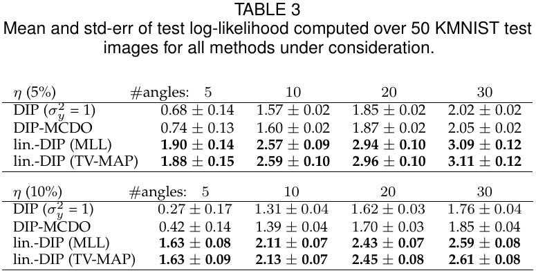
python exact_density.py experiment=kmnist num_images=50 use_double=True inference.load_path=$OUTPUT_LIN_DIP trafo.num_angles=20 dataset.noise_stddev=0.05

Here, covariances between all image pixels are considered (not only those inside patches like for the Walnut).

The following table shows numerical results, benchmarking against DIP-MCDO (see experiments/run_baselines_mcdo.py and experiments/run_baselines_density.py) and a simple Gaussian noise model denoted by DIP (σ_y²=1).

Setup environment

We recommend using a conda environment, which can be created with

conda create -n bayes_dip -f environment.yml

Note that this includes optional development dependencies (tensorboard, pytest).

The astra-toolbox>=2.0.0 dependency is currently only available as a conda package, but not as a pip package (the version is outdated).

Citation

If you find this code useful, please consider citing our paper:

Javier Antorán, Riccardo Barbano, Johannes Leuschner, José Miguel Hernández-Lobato & Bangti Jin. (2022). Uncertainty Estimation for Computed Tomography with a Linearised Deep Image Prior.

@misc{antoran2022bayesdip,
    title={Uncertainty Estimation for Computed Tomography with a Linearised Deep Image Prior},
    author={Javier Antorán and Riccardo Barbano and Johannes Leuschner and José Miguel Hernández-Lobato and Bangti Jin},
    year={2022},
    eprint={2203.00479},
    archivePrefix={arXiv},
    primaryClass={stat.ML}
}