Multifidelity global sensitivity analysis

Repository overview

This code implements the multifidelity approach to estimating variance and global sensitivity indices as described in:

1. Qian, E., Peherstorfer, B., O'Malley, D., Vesselinov, V., and Willcox, K. Multifidelity Monte Carlo Estimation of Variance and Sensitivity Indices. SIAM/ASA Journal on Uncertainty Quantification, 6(2):683-706, 2018.

   BibTeX

   @article{qian2018multifidelity,
   title={Multifidelity {M}onte {C}arlo estimation of variance and sensitivity indices},
   author={Qian, Elizabeth and Peherstorfer, Benjamin and O'Malley, Daniel and Vesselinov, Velimir V and Willcox, Karen},
   journal={SIAM/ASA Journal on Uncertainty Quantification},
   volume={6},
   number={2},
   pages={683--706},
   year={2018},
   publisher={SIAM}
   }

2. Cataldo, G., Qian, E., and Auclair, J. Multifidelity uncertainty quantification and model validation of large-scale multidisciplinary systems. Journal of Astronomical Telescopes, Instruments, and Systems, 8(3):038001, 2022.

   BibTeX

   @article{cataldo2022multifidelity,
   title={Multifidelity uncertainty quantification and model validation of large-scale multidisciplinary systems},
   author={Cataldo, Giuseppe and Qian, Elizabeth and Auclair, Jeremy},
   journal={Journal of Astronomical Telescopes, Instruments, and Systems},
   volume={8},
   number={3},
   pages={038001},
   year={2022},
   publisher={SPIE},
   doi = {10.1117/1.JATIS.8.3.038001},
   URL = {https://doi.org/10.1117/1.JATIS.8.3.038001}
   }

Two examples from [1] are provided:

• The ishigami folder contains everything needed to run the numerical experiments for the analytical Ishigami function example. This is a baseline example for implementing our multifidelity estimation strategy when you can evaluate your functions at different inputs in real time.
• The CDR folder contains the samples needed to run the numerical experiments for the convection-diffusion-reaction example. This is a baseline exmaple for implementing our multifidelity estimation strategy when you have to precompute your samples and bootstrap from the pre-computed sample for sensitivity index estimation.

Further, main_ishi.m in the ishigami folder allows the use of the rank-statistics-based estimators from Gamboa et al. 2020, as described in [2].

Global sensitivity analysis

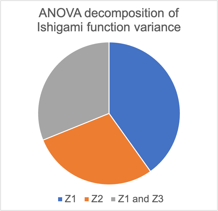
When a model has uncertain inputs, the model output is also uncertain. Variance-based global sensitivity analysis quantifies the relative influence of each of these uncertain inputs on the output by dividing the total variance into percentages of the variance due to each of the inputs and due to interactions between inputs. For example, the Ishigami function has 3 random inputs, Z₁, Z₂, and Z₃, each distributed uniformly on the interval [-𝜋,𝜋]:

The variance of the Ishigami function can therefore be decomposed into the variance components that are due to the influence of input 1 alone, input 2 alone, input 3 alone, or the interactions between inputs 1 and 2, inputs 1 and 3, or inputs 2 and 3, or finally due to interactions between all three inputs. This decomposition is known as the analysis-of-variance (ANOVA) decomposition, and amounts to decomposing the variance 'pie' into slices of pie. For the above Ishigami function (with a = 5 and b = 0.1), 40% of the variance is due to Z₁ alone, 29% of the variance is due to Z₂ alone, and 31% of the variance is due to the interaction between Z₁ and Z₃. Thus, here is what the variance pie looks like:

Global sensitivity indices quantify how much of the variance pie can be attributed to each input. For a given input, there are two different global sensitivity indices:

• the main effect sensitivity index, which represents the percentage of variance that can be attributed to that input alone, i.e. effects due to interactions between that input and others are not accounted for, and
• the total effect sensitivity index, which represents the total percentage of variance that is influenced by that input, including effects due to that input alone, as well as effects due to that input and other inputs.

In general, the sum of the main effect sensitivities for all inputs adds to 1 or less, while the sum of the total effect sensitivities adds to 1 or greater. For example, in the above Ishigami function example, the main effect sensitivity indices for Z₁, Z₂, and Z₃, respectively, are 0.40, 0.29, and 0, respectively, while the total effect sensitivity indices are 0.71, 0.29, and 0.31, respectively.

Monte Carlo sensitivity index estimation and multifidelity strategy

The main and total effect sensitivity indices can be estimated using Monte Carlo estimation. To estimate both the main and total effect sensitivity indices for d inputs, (d+2) function evaluations per Monte Carlo sample are required, so that the Monte Carlo estimation can be very expensive when the model is expensive and d is large. We propose multifidelity estimators which combine a few high-fidelity samples, computed using the expensive model, with many low-fidelity samples, computed using cheaper surrogate models, to yield lower-variance estimates for a fixed computational budget than would be obtained using the high-fidelity model alone, while retaining the accuracy of the high-fidelity estimate.

Related papers

• Peherstorfer, B., Willcox, K., and Gunzburger, M. Optimal model management for multifidelity Monte Carlo estimation. SIAM Journal on Scientific Computing, 38(5):A3163-A3194, 2016. (MFMC GitHub)
• Gamboa, F., Gremaud, P., Klein, T., and Lagnoux, A. Global sensitivity analysis: A new generation of mighty estimators based on rank statistics, 2020.

Contact

Please feel free to contact Elizabeth Qian with any questions about this repository or the associated paper.