
Grav Mag Suite is an open source MATLAB-based package for processing potential field geophysical data. The codes are written in MATLAB (version 9.4.0.813654 R2018a). This project partially represents the final product of the master degree programme of Federal University of Paraná [UFPR] in collaboration with Laboratory for Research in Applied Geophysics [LPGA].
Most geophysical software/suites are comercial or just simple open source command line programs. With Grav Mag Suite the user have in hand a variety of tools capable of perform several kinds of processing tasks over potential field geophysical data. To make it easier, every processing tool has a corresponding graphical user interface (GUI) which allows the user to perform processing tasks in few steps. In this way, Grav Mag Suite gathers the best of two worlds: be open source and easy to operate.
- Fabrício Rodrigues Castro [fcastrogeof@gmail.com].
Connect with me at LinkedIn.
- Youtube Channel -> Grav Mag Suite YouTube Channel
- Saulo Pomponet Oliveira [saulopo@ufpr.br].
- Jeferson de Souza [jdesouza@ufpr.br].
- Francisco José Ferreira Fonseca [francisco.ferreira@ufpr.br].
Grav Mag Suite may be installed by copying the content of the compressed file [Grav Mag Suite.rar] into a directory of your choice.
IMPORTANT!
To work properly, Grav Mag Suite must be executed using the following version of MATLAB -> (version 9.4.0.813654 or R2018a). Older or newer MATLAB versions may trigger some issues.
In order to maintain the program more stable your feedback is very important. Then, if you are facing any issue please report your bug sending me an E-mail at [fcastrogeof@gmail.com].
(click to expand!)
Profile Analysis (click to expand!)
 This tool allows to load a profile [2 columns ASCII file] and apply some enhacement filters (ASA, THDR, TDX, TDR, among otherS) as well as derivative filters (both vertical and same direction of profile).
Extract Profile From a Grid (click to expand!)


In this GUI a grid file can be loaded and it's possible to extract a profile from it. There are three modes of profile extraction:
- One can extract an entire row or column from grid;
- The user can extract a profile by drawing a single line or polyline over the grided map;
- The user can load a control file in .ply format that contains coordinate pairs representing vertices of a path and extract the values over it.
Obs.: In this tool a gridded file (regularly spaced) must be loaded to work properly. Avoid load scattered data.
(click to expand!)
Derivative Filters (click to expand!)


Directional Derivative Filter (click to expand!)


Generalized Derivative Operator (click to expand!)


More details about this operator is found at: Cooper & Cowan, 2011
Vertical Derivative using Upward Continuation (click to expand!)


Field Continuation (click to expand!)


Directional Cosine (click to expand!)


Change Direction of Measurement (click to expand!)


Reduction to the Pole (RTP) (click to expand!)
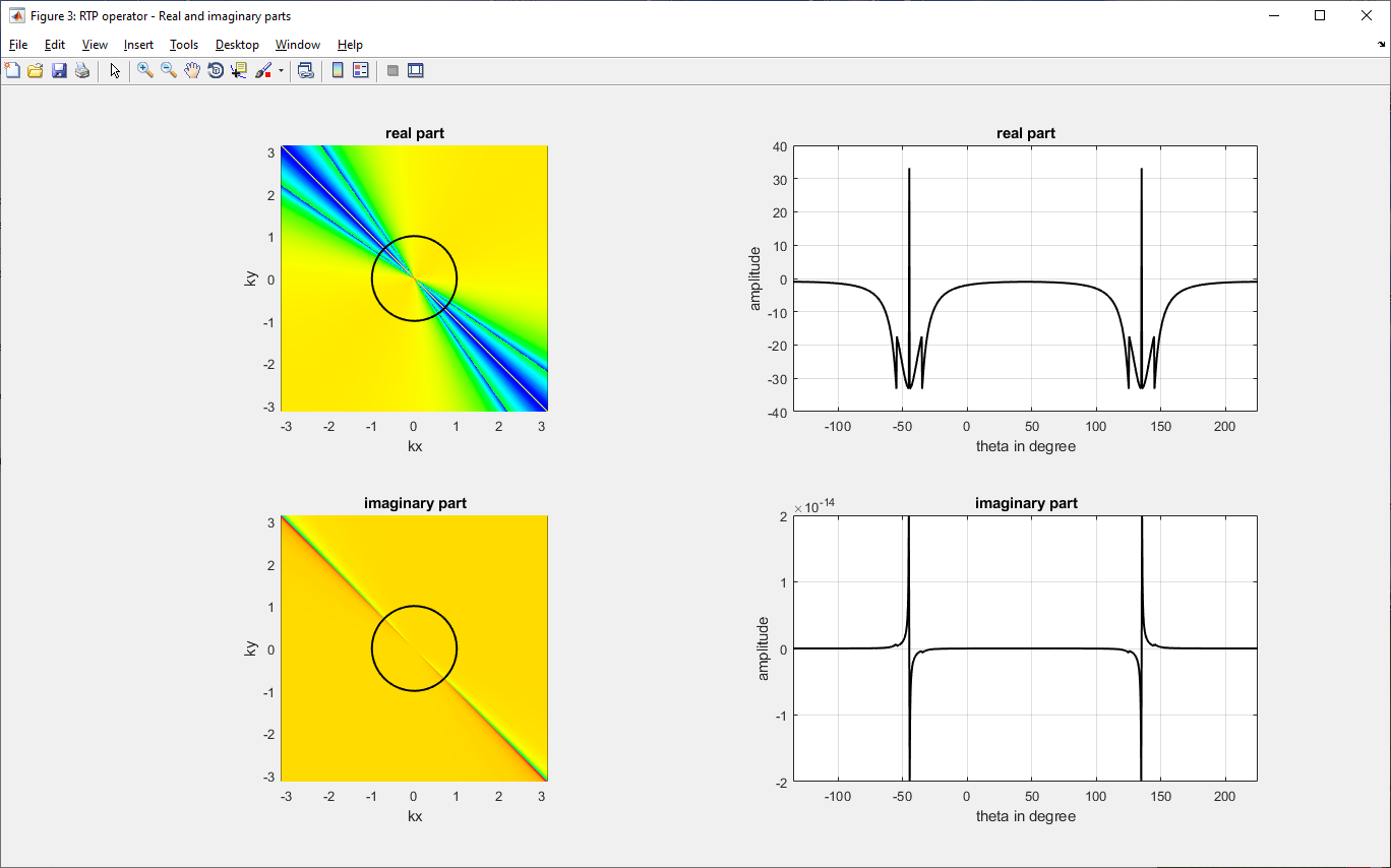
The reduction to the pole GUI can reduce the input data under 3 different approaches, Pseudo-inclination (MacLeod et al. 1993), Azimuthal filtering (Phillips, 1997), and Nonlinear thresholding (Zhang et al. 2014). Once an approach is choosen, the GUI components related to the selected RTP method will be visible.

-
Pseudo Inclination Method.
The RTP wavenumber-domain operator is expressed by the following equation:
or in polar coordinates (with r=1):In the pseudo-inclination approach, the above RPT operator is used normally, but at unstable zones (D+90-beta<theta<D+90+beta and D+270-beta<theta<D+270+beta) the bellow expression is used instead:
where (I_a) is an user-given parameter called pseudo-inclination. It must be larger than the actual magnetic inclination (I) and its absolute value may often be between 20 and 30 degrees. The following figures show a TMI anomaly with (I=1 and D=45) and its reduced to the pole product, and both real and imaginary parts of the RTP operator, showing that its amplitudes at unstable zones were fairly atenuated.

Reduction to the Equator (RTE) (click to expand!)


Vertical Integration (click to expand!)


Hilbert Transform (click to expand!)
![]()

Anisotropic Diffusion Filter (click to expand!)
Other Filters (click to expand!)
- Convolutional Filters:


- Fourier Domain Filters:


(click to expand!)
Classical Enhancement Filters (click to expand!)


Balanced Horizontal Derivative [Edge Detector] (click to expand!)


For more information visit -> Ma and Li, 2014.
Monogenic Signal (click to expand!)


For more information visit -> Hidalgo Gato and Barbosa, 2015 and Hidalgo Gato and Barbosa, 2017.
Normalized Standard Deviation (click to expand!)


For more information visit -> Cooper and Cowan, 2005.
Vertical Integration of ASA (click to expand!)


For more information visit -> Paine and Haederle, 2001.
TDR+-TDX (click to expand!)


(click to expand!)
Source Distance (click to expand!)
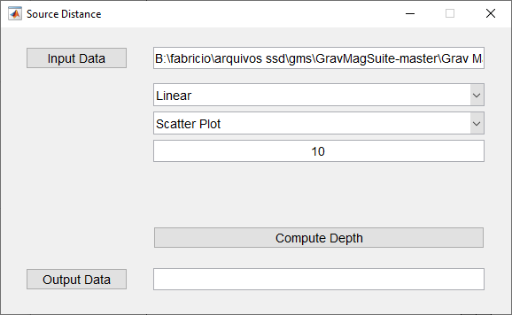
This semiquantitative method has two ways of represent the estimated depth, in a surface map or in a scattered plot.
- Surface map;

- Scattered plot;


Tilt-Depth (click to expand!)

This semiquantitative method displays the following products: input data, TDR, depth estimates in scattered plot, and histogram of depth estimates.


Signum Transform (click to expand!)
![]()


For more information visit -> Souza & Ferreira, 2015 and Weihermann et al. 2016.
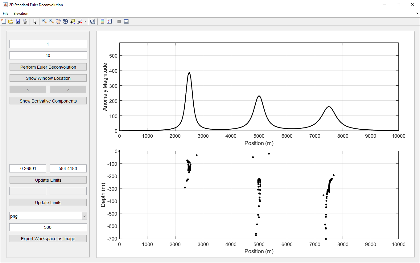
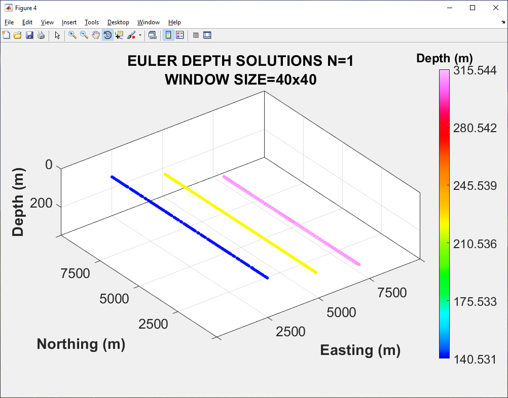
Euler Deconvolution (click to expand!)
- Bidimensional:
- Tridimensional [Moving window approach]:

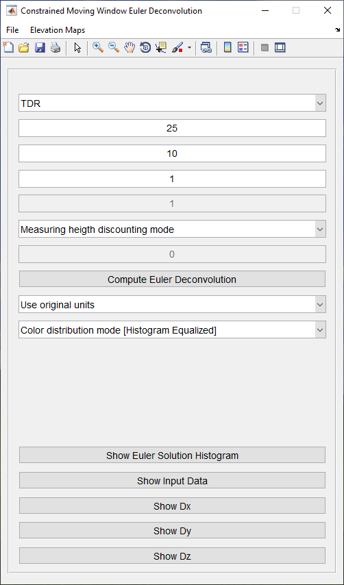
- Tridimensional [Constrained moving window approach]:

Scattered Solution Tools (click to expand!)
- Plot Scattered Solutions:

- Histogram Classes Separation:


- Subset Solutions:


(click to expand!)
2D Modeling (click to expand!)
Spherical Body (click to expand!)

Dyke-Like Body (click to expand!)

Fault Model (click to expand!)

Irregular Cross-Section Body (click to expand!)

3D Modeling (click to expand!)
-
Prismatic Body:
This GUI is composed by 4 fields: a left-side panel, a upper-right graph, a down-right parameter table, and an uppermost menu.
-
Left-side panel: It's composed by several UI components like, entries, popupmenus, and buttons. The first two lines of the panel have entry components related to the interpolation mesh. The third line is composed by 3 entries related to magnetic inducing field strength, inclination, and declination, and the fourth line represents entries related to magnetic and gravity noise level. The fifth and sixth lines are composed by popup menus that control the way that the calculated anomaly will be shown. The user can choose to display the magnetic or the gravity anomaly, and choose to show it in the 2D or 3D form, as well as choose the color distribution to be linear or histogram equalized. The first line of the left-side panel's bottom entries has two UI components that set the quantity of bodies that the model is composed. When the user pic a number and press the ok button, some empty columns will appear in the down-right parameter table. Each column is related to a body. The next 2 lines of the left-side panel represet entries that set a filename sufix used to differentiate the magnetic from the gravity anomaly file. The "compute the anomalies" button as the name suggests calculate both gravity and magnetic anomalies. When the user press this button, a dialogue window will popup asking the user to choose both directory and file name, where the anomaly files will be saved. The last 3 lines of the left-side panel will set the way the model will be displayed. The user can set to show the entire bodies of the model in case of bodies limits exceed the study area limits and can set the vertical range (depth interval) of the model.
-
Upper-right graph: This part of the GUI is intended for displaying the calculated anomaly maps.
-
Down-right parameter table: In the parameter table the user can set both physical and spatial parameters of model's bodies, like magnetic susceptibility, density, remanet intensity, inclination and declination, width, lenght, thickness of the body, as well as depth to the top, and strike azimuth.
-
Uppermost menu: In this menu there are 2 options to load and save a control file related to the model's configuration. When the user load a model control file, several UI components will be automatically set with the info saved in the loaded file. Or, when the user save a control file, all model's info present in the GUI will be saved.
The bellow figures represents the GUI and the model used in the forward modeling.
-


- Spherical Body:

