3 Video visualization
Videos can be watched as they are, but they can also be used to develop new visualisations to be used for analysis. The aim of creating such alternate displays from video recordings is to uncover features, structures and similarities within the material itself, and with, for example, score material. Here are three useful visualisation techniques: motion images, motion history images and motiongrams.
MGT can generate both dynamic and static visualizations, as well as some quantitative data:
- dynamic visualisations (video files)
- motion video
- motion history video
- static visualisations (images)
- motion average image
- motiongrams
- videograms
- motion data (csv files)
- quantity of motion
- centroid of motion
- area of motion
In the following, we will try this ourselves and look at the different types.
The easiest way to get started with analysing video with MGT is by just running the function mgmotion. In Matlab, you need to ensure that you are in the "examples" working directory.
Then you can write the following to run the mgmotion function on the video file dance.avi:
mgmotion('dance.avi');
This will generate four files in the same location as your source file:
- dance_motion.avi: the motion video that is used as the source for the rest of the analysis
- dance_mgx.tiff: a horizontal motiongram
- dance_mgy.tiff: a vertical motiongram
- dance_data.csv: a data file with some quantitative features
- dance_com_qom.eps: an image file with plots of centroid and quantity of motion
We will examine each of these in a little more detail.
The analysis covered in this part is based on a widespread video analysis technique called "frame differencing". Here we create a motion image by calculating the absolute pixel difference between subsequent frames in the video file:
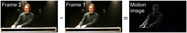
The result is an image where only the pixels that have changed between the frames are displayed. This can be interesting in itself, but motion images are also the starting point for many other video visualisation and analysis techniques.
A motion video is a series of motion images, showing only the motion happening between the two last frames in the original video file.
Matlab does not have an easy and universal approach of adding audio streams to exported video files. So if you want audio on your motion video, it is better to do that outside of Matlab, using FFmpeg. This oneliner will do the trick:
ffmpeg -i dance.avi -i dance_motion.avi -c copy -map 1:v:0 -map 0:a:0 -shortest -c:v mpeg4 -c:a aac dance_motion_audio.mp4
Here we output to a compressed .MP4 file, a great format for video that is primarily meant for watching (not further analysis).
If you think there is too much noise in the output images or video, you may choose to use some other filter settings. Try this:
mgmotion('dance.avi','Diff','Regular',0.1);
Here a filter setting of 0.2 is used instead of 0.1. The number goes between 0 and 1, where 0 will let through all pixels, while 1 will only let through completely white pixels. The default setting is 0.1, and this usually works quite well for most videos. If you want more detail, you can try setting it down to 0.05, or if you have too much noise, you can raise it to 0.2 or 0.3.
The two other settings above refer to the type of motion analysis we are doing (OpticalFlow is another option, which we will look at towards the end) and the type of filter we are using (Binary will output a black/white video as opposed to greyscale). Try, for example:
mgmotion('dance.avi','Diff','Binary',0.2)
Please note that every time you run the mgmotion function on the same file, it will overwrite the previous run's output. So if you want to keep differently filtered versions, you need to rename them. It may also be beneficial to copy the output files into a separate folder in which you specify the different settings you used.
You can always ask Matlab for help with any command, for example like this:
help mgmotion
which will tell you about the different options and settings.
While a motion history image may reveal information about a motion sequence's spatial aspects over a fairly short period of time, it is possible to use a motiongram to display longer sequences. This display is created by plotting the normalised mean values of the rows of a series of motion images. The motiongram makes it possible to see both the location and quantity of motion of a video sequence over time and is thus an efficient way of visualising longer motion sequences.
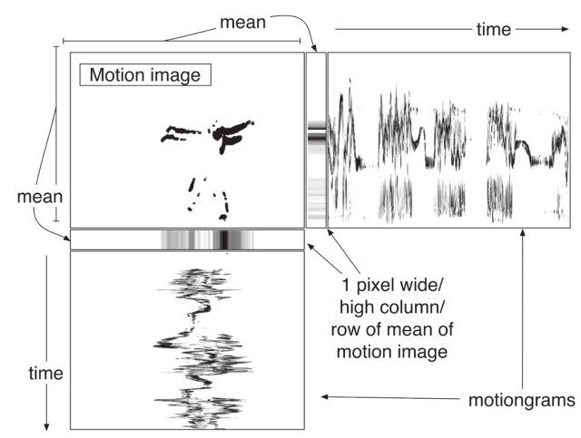
A motiongram is only a reduced display of a series of motion images, with no analysis being done. It might help to think of the motiongram as a display of a collapsed series of pictures, or “stripes,” where each “stripe” summarises a whole motion image's content.
Dependent on the video file's frame rate, motiongrams can be created from recordings as short as a few seconds to several hours. Short recordings can follow detailed parts of a body, particularly if there are relevant colours in the image. In contrast, motiongrams of longer recordings will mainly reveal larger sections of motion. Motiongrams work well together with audio spectrograms and other types of temporal displays such as graphs of motion or sound features.
If you look at the content of dance.csv, it contains numbers like this:
1.2162e+05,259.1,223.2
97576,256.26,210.92
88415,250.04,214.91
76769,249.61,221.22
81350,242.81,218.21
77598,239.7,208.27
70974,256.93,219.15
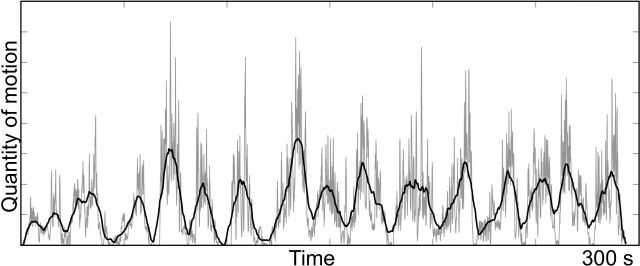
Here the first column contains the quantity of motion (QoM), which is the sum of active pixels in the image. The two next columns include the x and y values for the centroid of motion. The exported plot dance_motion_com_qom.eps gives you an idea of how the data looks like. The data are also available for further calculation and plotting (as we will get back to later).
The broad field of computer vision is concerned with extracting useful information from video recordings. Some basic motion features that are commonly used in music research are derived directly from the motion image. Since the motion image only shows pixels that have changed between the two last frames in a video sequence, the sum of all these individual pixels' values will give an estimate of the quantity of motion (QoM). Calculating the QoM for each frame will give a numeric series that can be plotted and used as an indicator of the activity.
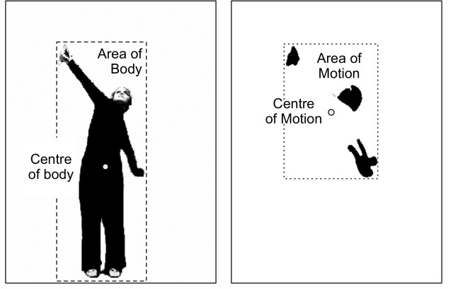
The centroid of motion (CoM) and area of motion (AoM) are other basic features that can easily be extracted from a motion image, and the differences between them are illustrated in Figure [fig:37-com]. The CoM and AoM features can be used to illustrate where in an image the motion occurs and the spatial displacement of motion over time.
While motiongrams are good for getting a general sense of a video file's spatiotemporal distribution, a motion average image is good for getting a general sense of the space covered. This may be thought of as similar to an "open shutter" on a camera, since the function just averages (and normalizes) over all the frames. Try:
mgmotionaverage('dance_motion.avi');
If the motion is evenly distributed in the image, the motion average image may not contain much information. But if a person has been standing still in one spot, it will show up very clearly.
It is also possible to run this function on the original video:
mgmotionaverage('dance.avi');
Such an average image may also be useful in combination with the motion average image.
If you only want to look at a particular part, you may choose to identify the start and stop positions of the averaging (in seconds from the start of the file):
mgmotionaverage('dance.avi',0,5);
So here we get the average of the first 5 seconds of the file.
One dynamic visualization technique is creating a motion history video, which gives you an idea of how the movement has been unfolding in time. This can be done with the following command:
mgmotionhistory('dance_motion.avi');
It can, in fact, also be run on the original video:
mgmotionhistory('dance.avi');
We have up until now primarily worked with video in greyscales. This is more CPU-friendly since it only consumes 1/4 of the processing power as that of colour. Sometimes colour may be important, though, so it is possible to run the process on all the video planes like this:
mgmotionhistory('dance.avi',20,'color');
The number 20 here refers to the number of frames of history. You can try some different settings here too.