Handling schedules and Gantt charts
scheptk includes the class Schedule, which can be used to save, load and print schedules that can be generated by the supporting scheduling layouts, or can be also generated autonomously by adding tasks to an existing schedule.
A typical schedule file is a text file containing the following tags:
[JOBS=5]
[MACHINES=4]
[SCHEDULE_DATA=1,0,10,0,10,10;1,10,20,2,40,20;2,80,120;1,30,10;3,30,10]
[JOB_ORDER=0,1,2,3,4]
The tag JOBS indicates the number of jobs in the schedule, MACHINES the number of machines, and SCHEDULE_DATA contains the tasks for each job (in the order given by JOB_ORDER) in the form of a tuple machine, starting_time, duration.
Different methods can be used to handle schedules. These are described in the next subsections
A schedule stored in a file sched.sch can be open using the constructor of the class Schedule. If no argument is specified, an empty instance of the Schedule class is created. The following code opens and print the schedule contained in the file openshop.sch
from scheptk.scheptk import Schedule

sched = Schedule('openshop.sch')
sched.print()If the schedule has been generated autonomously, or is contained in an instance of the class Schedule, it can be saved using save(filename).
from scheptk.scheptk import Schedule, Task

gantt = Schedule()

gantt.add_task(Task(0,0,10,20))
gantt.add_task(Task(0,1,0,10))
gantt.add_task(Task(1,1,10,30))
gantt.add_task(Task(1,2,40,60))

gantt.save('resulting_schedule.sched')
A schedule obtained from a given instance using a solution sol, it can be saved using the method write_schedule(sol, filename).
from scheptk.scheptk import OpenShop

instance = OpenShop('test_openshop.txt')
sol = [7,5,4,0,1,6,3,2,8]
instance.write_schedule(sol, 'openshop.sch')
Alternatively, the method create_schedule(solution) can be used to get the corresponding schedule and then saving it using the save() method of the class Schedule as seen before.
from scheptk.scheptk import OpenShop

instance = OpenShop('test_openshop.txt')
sol = [7,5,4,0,1,6,3,2,8]
gantt = instance.create_schedule(sol)
gantt.save('openshop.sch')Use the method print() in the class schedule. A filename to store the image can be specified optionally:
from scheptk.scheptk import Schedule, Task

gantt = Schedule()

gantt.add_task(Task(0,0,10,20))
gantt.add_task(Task(0,1,0,10))
gantt.add_task(Task(1,1,10,30))
gantt.add_task(Task(1,2,40,60))

gantt.print()
If the schedule is to be generated from a solution in a given layout, you can use the method print_schedule(solution) of the corresponding layout
from scheptk.scheptk import FlowShop
instance = FlowShop("test_flowshop.txt")
sequence = [0,1,4,3,2]
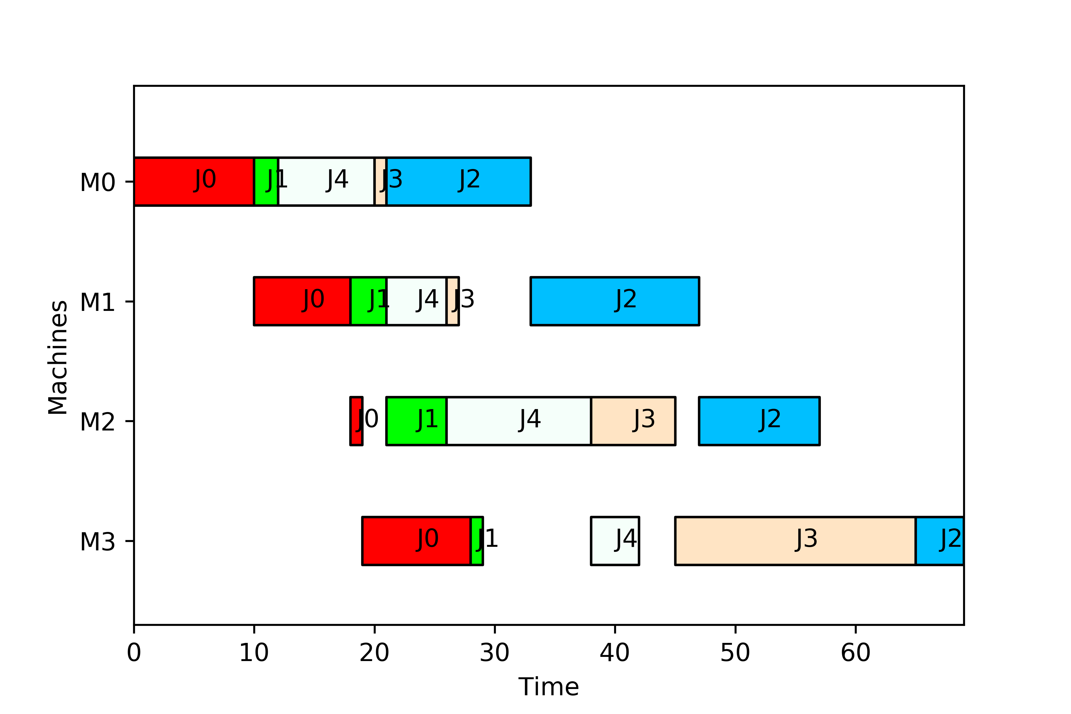
instance.print_schedule(sequence, 'flowshop_sample.png')The following image is printed:
Alternatively, use create_schedule() to first obtain the schedule and later print it with the print() method, i.e.
from scheptk.scheptk import FlowShop
instance = FlowShop("test_flowshop.txt")
sequence = [0,1,4,3,2]
gantt = instance.create_schedule(sequence)
gantt.print('flowshop_sample.png')A schedule can be created by adding tasks to an instance of the class Schedule. The tasks are added using the method add_task(), which takes as argument an instance of the class Task. The constructor of the class Task requires four arguments, i.e. Task(job, machine, st, ct) where job and machine indicates the job and the machine whereas st and ct indicate the starting and completion times of the task, respectively. The following code creates an empty schedule, then it populates it with several tasks and finally prints the resulting schedule:
from scheptk.scheptk import Schedule, Task

gantt = Schedule()

gantt.add_task(Task(0,0,10,20))
gantt.add_task(Task(0,1,0,10))
gantt.add_task(Task(1,1,10,30))
gantt.add_task(Task(1,2,40,60))
gantt.add_task(Task(2,2,80,200))
gantt.add_task(Task(3,1,30,40))
gantt.add_task(Task(4,3,30,40))


gantt.print('figure.png')
The schedule generated is the following:

In general, a Schedule shows a Gantt chart with the evolution of the state of the machines in the layout over the time. There are three basic states for a machine in a given time:
- The machine may be busy while processing a job. This time period is denoted as a
Taskfor the machine. - The machine may be idle as there are no available jobs to be processed. This time period is represented in the Gantt chart by a void.
- The machine may be unavailable for processing a job (even if the job is available) as a set-up operation, maintenance process, breakdown, or another incidence makes the machine unavailable. This time period is denoted as
NAP(Non Availabiliy Period) :-)

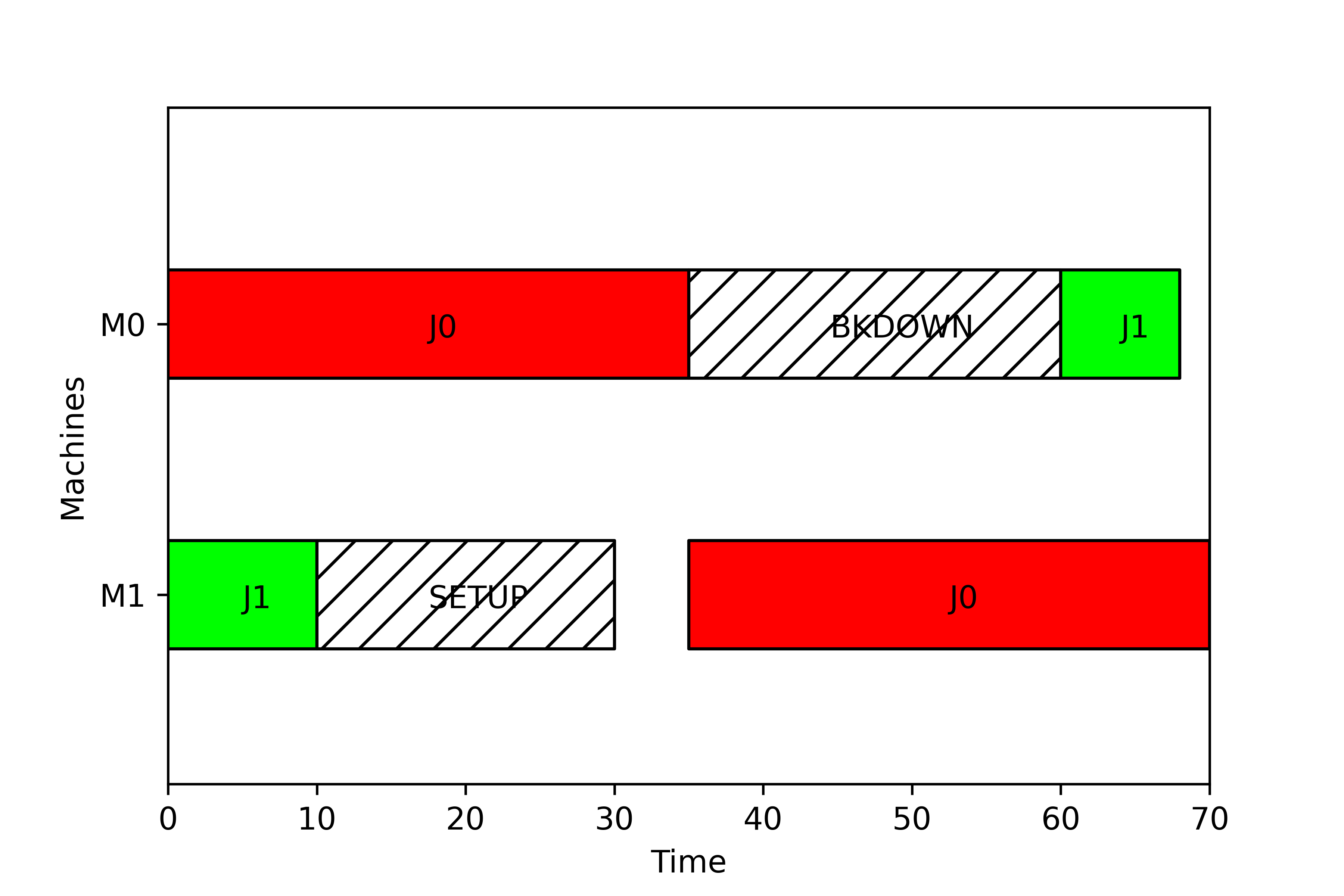
In the figure we can see the three periods in a SingleMachine layout. From period 0 to 10 the machine is idle (in this case it is because the job has a release date of 10 units). From period 10 to 48 the machine is processing J2. From period 48 to 73 there is a setup of 25 time units in order to prepare the tool from J2 to J0, and from time 73 to 93, job 0 is processed.
These elements can be implemented in scheptk adding to an existing Schedule object elements from the classes Task and NAP. In most cases, both objects are only using to give information to the schedule about the task and the NAP. The following line
new_task = Task(job_index, machine_index, st, ct)
creates a new task (named new_task) that processes job job_index on machine machine_index from time st to time ct. Analogously, the following line
new_nap = NAP(machine_index, st, ct, nap_tag)
creates a new NAP (named new_nap) where the machine machine_index is not available from time st to time ct. Optionally, the tag nap_tag will be set in this NAP when printing the Gantt diagram. The following complete code
from scheptk.scheptk import Task, NAP, Schedule

gantt = Schedule()
# tasks and NAP for machine 0
gantt.add_task(Task(0,0,0,35))
gantt.add_NAP(NAP(0,35,60,'BKDOWN'))
gantt.add_task(Task(1,0,60,68))

# tasks and NAP for machine 1
gantt.add_task(Task(1,1,0,10))
gantt.add_NAP(NAP(1,10,30,'SETUP'))
gantt.add_task(Task(0,1,35,70))

# printing the schedule
gantt.print()
creates tasks and NAP and add them to the schedule in the figure
Clearly, the idea of the Tasks and NAPs is not to be used in an isolated manner, but to integrate them into a (possibly customised) scheduling model. As it has been discussed in Section , to obtain a customised scheduling model, it is only required to create a child class of the class Model and to write the specific code for the constructor method (where the data required are defined) and for the ct method (where the completion times for each job in a given job order are computed). In addition, to include a customised Gantt chart, we would also need to overwrite the parent method print_schedule, as this method in the class Model does not consider NAPs. To illustrate the whole process, in this section we will present a single machine scheduling model with sequence-dependent setup and release times. This new model (named SingleMachineSetUp) not only will compute the usual scheduling criteria, but also will print a schedule that takes into account the sequence-dependent setups. The full code for this model is the following:
from scheptk.scheptk import Model, NAP
from scheptk.util import *

class SingleMachineSetUp(Model):

    # constructor
    def __init__(self, filename):
        self.jobs = read_tag(filename,'JOBS')
        self.pt = read_tag(filename,'PT')
        self.sj = read_tag(filename,'SJ')
        self.r = read_tag(filename,'R')

    # compute completion times (assumed anticipatory setup)
    def ct(self, solution):
        ct = [0 for j in range(len(solution))]
        ct[0] = max(self.r[solution[0]],self.sj[solution[0]][solution[0]]) + self.pt[solution[0]]
        for j in range(1,len(solution)):
            ct[j] = max(self.r[solution[j]],ct[j-1] + self.sj[solution[j]][solution[j-1]]) + self.pt[solution[j]]
        return [ct], solution

    # print customised schedule
    def print_schedule(self, solution, filename=None):
        completion_time, sol = self.ct(solution)
        gantt = Model.create_schedule(self,solution)
        gantt.add_NAP(NAP(0,0, self.sj[solution[0]][solution[0]],'SETUP'))
        for j in range(1,len(solution)):
            st = completion_time[0][j] - self.pt[solution[j]] - self.sj[solution[j]][solution[j-1]]
            gantt.add_NAP(NAP(0,st, st + self.sj[solution[j]][solution[j-1]],'SETUP'))
        gantt.print(filename)
As we can see, a SingleMachineSetUp class has been defined as a child of the parent class Model. This allows SingleMachineSetUp to use all methods for scheduling layouts once we provide an specific way to enter the data and to compute the completion times from this data. The data of the model are described in the constructor __init__(self, filename), where the data are jobs (an integer indicating the number of jobs), pt (an array indicating the processing time of each job), r (an array with the release date of each job), and sj, which requires a more detailed explanation. Although there are different possibilites --after all, it is a customised model so we define which data are required and how are used--, we define sj as a two-dimensional array. In this manner sj[k][l] indicates the setup time required when job l is processed immediately after job k. To model the need to introduce a setup time if no prior job has been entered in the sequence, sj[k][k] would contain this initial setup time.
With the constructor method, an instance data file would look like this
[JOBS=3]
[PT=20,35,38]
[R=10,10,10]
[SJ=0,12,25;5,40,2;30,12,0]
So in this instance there are three jobs (with processing times 20, 35 and 38 respectively, and release times 10, 10 and 10), and the setup times are as follows:
| Job/job | 0 | 1 | 2 |
|---|---|---|---|
| 0 | 0 | 12 | 25 |
| 1 | 5 | 40 | 2 |
| 2 | 30 | 12 | 0 |
which means that, if job 1 is processed immediately after job 0, then a setup time of 5 units is required.
The second method (ct) computes the completion times. Remember that the method takes as input a solution of the problem, and returns the completion times on each machine, and the order in which the completion times of the jobs are given. In our case, a solution would be a (maybe partial) list of jobs, so sol = [2,0,1] would indicate that job 2 is processed first, next job 0, and finally job 1.
The first line in the ct method simply creates a list with the completion times of the jobs entered in the solution, and initially these completion times are zero. Next, for the first job, it simply computes the completion time as ct[0] = max(self.r[solution[0]],self.sj[solution[0]][solution[0]]) + self.pt[solution[0]], i.e. the completion time of the first job is the maximum between the release date of the job and its initial setup time plus the processing time of the job. Next is a loop where the completion time of the other jobs are computed. In this case, the completion time is the maximum between the release date of the job and the completion time of the previous job in the machine plus the setup time required plus the processing time of the job. The method returns the completion time of each job in the solution and the order in which the jobs are described in the completion times.
In principle, with this two methods would be sufficient to compute the usual criteria. If the following code is produced (using the instance data file single_setup.txt provided above)
from scheptk.scheptk import Model, NAP
instance = SingleMachineSetUp('single_setup.txt')
solution = [2,0]
print('Makespan=',instance.Cmax(solution))
print(solution)
then the makespan is correctly computed, but when the schedule is printed, there is a void of 25 periods between the processing time of job 0 and that of job 2. This void corresponds to the setup induced when job 0 is processed after job 2 (see setup matrix). If the setups are entered in the Scheduleas non-availability periods, then they could appear in the schedule. This is the goal of the third method (print_schedule). The first line of this method is to call the ct nethod to obtain the completion times (as later these completion times would be used). The second line simply calls the method create_schedule of the parent class Model. This line will create a standard schedule using the solution, that is, it will create all tasks corresponding to the solution without the NAPs. Then the NAPs are added to the schedule: the first line (gantt.add_NAP(NAP(0,0, self.sj[solution[0]][solution[0]],'SETUP'))) adds a NAP starting at time zero and finishing at the time required for the initial setup. The label of the NAP is SETUP. The rest of the non availability periods are added using a loop: the starting time is computed (completion time minus setup minus processing time), and then are added. The last line simply prints the schedule, now with all setup times properly set, as it can be seen in the figure.
By the way, the figure shows another feature related to printing the Gantt charts: if the NAPs are of zero length (as it happens with the job 2), then the NAP is not printed.