Modular Implementation of popular Deep Reinforcement Learning algorithms in Keras:
- Synchronous N-step Advantage Actor Critic (A2C)
- Asynchronous N-step Advantage Actor-Critic (A3C)
- Deep Deterministic Policy Gradient with Parameter Noise (DDPG)
- Double Deep Q-Network (DDQN)
- Double Deep Q-Network with Prioritized Experience Replay (DDQN + PER)
- Dueling DDQN (D3QN)
This implementation requires keras 2.1.6, as well as OpenAI gym.
$ pip install gym keras==2.1.6The Actor-Critic algorithm is a model-free, off-policy method where the critic acts as a value-function approximator, and the actor as a policy-function approximator. When training, the critic predicts the TD-Error and guides the learning of both itself and the actor. In practice, we approximate the TD-Error using the Advantage function. For more stability, we use a shared computational backbone across both networks, as well as an N-step formulation of the discounted rewards. We also incorporate an entropy regularization term ("soft" learning) to encourage exploration. While A2C is simple and efficient, running it on Atari Games quickly becomes intractable due to long computation time.
In a similar fashion as the A2C algorithm, the implementation of A3C incorporates asynchronous weight updates, allowing for much faster computation. We use multiple agents to perform gradient ascent asynchronously, over multiple threads. We test A3C on the Atari Breakout environment.
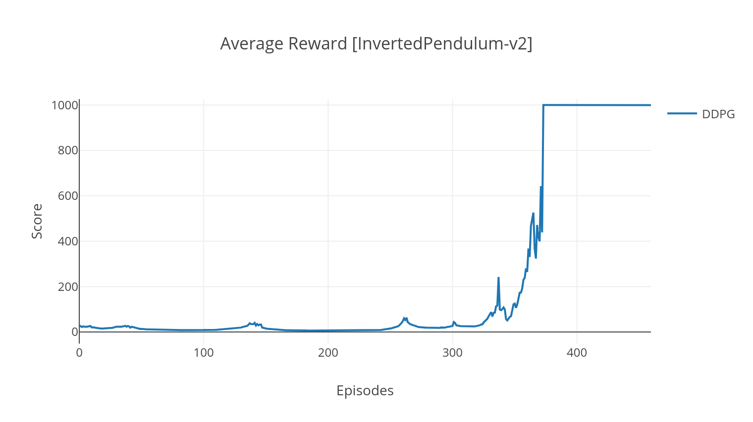
The DDPG algorithm is a model-free, off-policy algorithm for continuous action spaces. Similarly to A2C, it is an actor-critic algorithm in which the actor is trained on a deterministic target policy, and the critic predicts Q-Values. In order to reduce variance and increase stability, we use experience replay and separate target networks. Moreover, as hinted by OpenAI, we encourage exploration through parameter space noise (as opposed to traditional action space noise). We test DDPG on the Lunar Lander environment.
$ python3 main.py --type A2C --env CartPole-v1
$ python3 main.py --type A3C --env CartPole-v1 --nb_episodes 10000 --n_threads 16
$ python3 main.py --type A3C --env BreakoutNoFrameskip-v4 --is_atari --nb_episodes 10000 --n_threads 16
$ python3 main.py --type DDPG --env LunarLanderContinuous-v2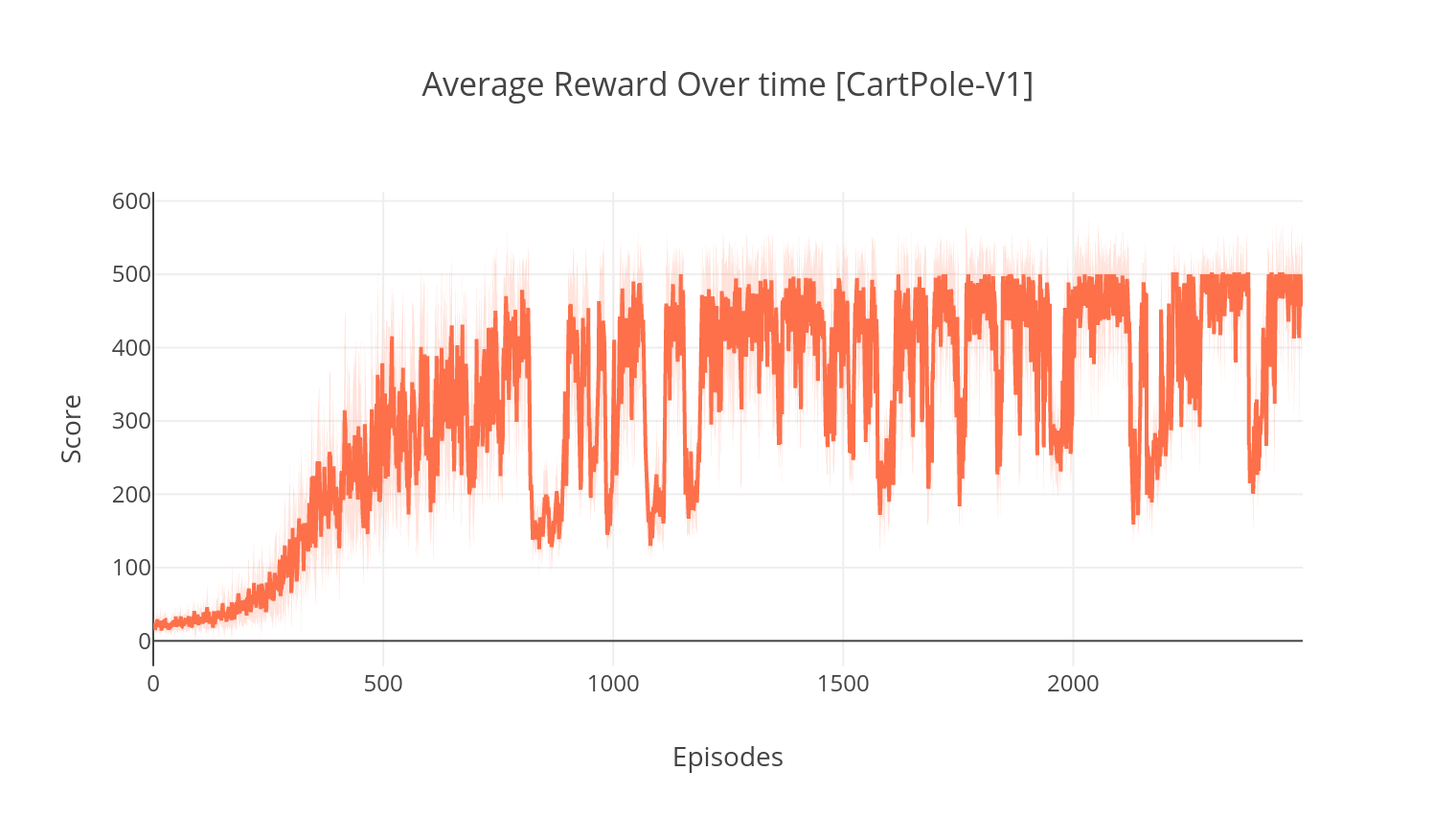
The DQN algorithm is a Q-learning algorithm, which uses a Deep Neural Network as a Q-value function approximator. We estimate target Q-values by leveraging the Bellman equation, and gather experience through an epsilon-greedy policy. For more stability, we sample past experiences randomly (Experience Replay). A variant of the DQN algorithm is the Double-DQN (or DDQN). For a more accurate estimation of our Q-values, we use a second network to temper the overestimations of the Q-values by the original network. This target network is updated at a slower rate Tau, at every training step.
We can further improve our DDQN algorithm by adding in Prioritized Experience Replay (PER), which aims at performing importance sampling on the gathered experience. The experience is ranked by its TD-Error, and stored in a SumTree structure, which allows efficient retrieval of the (s, a, r, s') transitions with the highest error.
In the dueling variant of the DQN, we incorporate an intermediate layer in the Q-Network to estimate both the state value and the state-dependent advantage function. After reformulation (see ref), it turns out we can express the estimated Q-Value as the state value, to which we add the advantage estimate and subtract its mean. This factorization of state-independent and state-dependent values helps disentangling learning across actions and yields better results.
$ python3 main.py --type DDQN --env CartPole-v1 --batch_size 64
$ python3 main.py --type DDQN --env CartPole-v1 --batch_size 64 --with_PER
$ python3 main.py --type DDQN --env CartPole-v1 --batch_size 64 --dueling
| Argument | Description | Values |
|---|---|---|
| --type | Type of RL Algorithm to run | Choose from {A2C, A3C, DDQN, DDPG} |
| --env | Specify the environment | BreakoutNoFrameskip-v4 (default) |
| --nb_episodes | Number of episodes to run | 5000 (default) |
| --batch_size | Batch Size (DDQN, DDPG) | 32 (default) |
| --consecutive_frames | Number of stacked consecutive frames | 4 (default) |
| --is_atari | Whether the environment is an Atari Game with pixel input | - |
| --with_PER | Whether to use Prioritized Experience Replay (with DDQN) | - |
| --dueling | Whether to use Dueling Networks (with DDQN) | - |
| --n_threads | Number of threads (A3C) | 16 (default) |
| --gather_stats | Whether to compute stats of scores averaged over 10 games (slow, see below) | - |
| --render | Whether to render the environment as it is training | - |
| --gpu | GPU index | 0 |
All models are saved under <algorithm_folder>/models/ when finished training. You can visualize them running in the same environment they were trained in by running the load_and_run.py script. For DQN models, you should specify the path to the desired model in the --model_path argument. For actor-critic models, you need to specify both weight files in the --actor_path and --critic_path arguments.
Using tensorboard, you can monitor the agent's score as it is training. When training, a log folder with the name matching the chosen environment will be created. For example, to follow the A2C progression on CartPole-v1, simply run:
$ tensorboard --logdir=A2C/tensorboard_CartPole-v1/When training with the argument--gather_stats, a log file is generated containing scores averaged over 10 games at every episode: logs.csv. Using plotly, you can visualize the average reward per episode.
To do so, you will first need to install plotly and get a free licence.
pip3 install plotlyTo set up your credentials, run:
import plotly
plotly.tools.set_credentials_file(username='<your_username>', api_key='<your_key>')
Finally, to plot the results, run:
python3 utils/plot_results.py <path_to_your_log_file>- Atari Environment Helper Class template by @ShanHaoYu
- Atari Environment Wrappers by OpenAI
- SumTree Helper Class by @jaara