Home

Ginkgo Performance Explorer User Guide

Note: this page was automatically generated by converting certain sections of the conference paper, and the tool got quite a few things wrong. This will be corrected in the near future.

This section provides a step-by-step user tutorial of GPE. Hands-on experience is enabled by accessing GPE on Ginkgo’s GitHub pages.[2] For those interested in extending the capabilities of the web application, the source code is also available on GitHub[3] under the MIT license.

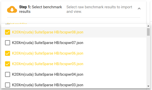The performance result selection pop-up dialog.

The web application is divided into three components, as shown in Figure [fig:web-app]. On the top left (and marked in red) is the data selection dialog. The dialog is used to retrieve the raw performance data from the performance repository. Clicking on the “Select result files” control opens a multiple select pop–up dialog listing available performance data. By default, the application uses Ginkgo’s performance data repository[4] to populate the list of available performance result files. However, an alternative performance database location (e.g. containing performance data for a different library) can be provided via the “Performance root URL”. The value of this control can be changed, and after clicking the download button on the right of the control, GPE will try to read the list.json file from the provided URL. This file lists the names and locations of the performance results. For example, if a database contains two data files located at “http://example.com/data/path/to/A.json” and “http://example.com/data/path/to/B.json,” then a “list.json” file with content structured like the following has to be available at “http://example.com/data/list.json”.

        [{
            "name": "A",
            "file": "path/to/A.json"
        }, {
            "name": "B",
            "file": "path/to/B.json"
        }]

Afterwards, the “Performance root URL” in GPE is changed to http://example.com/data, and the application will retrieve the data from the chosen location. Once the performance results are loaded, they can be viewed in the “Results” tab of the data and plot viewer (the blue box on the right-hand side in Figure [fig:web-app]).

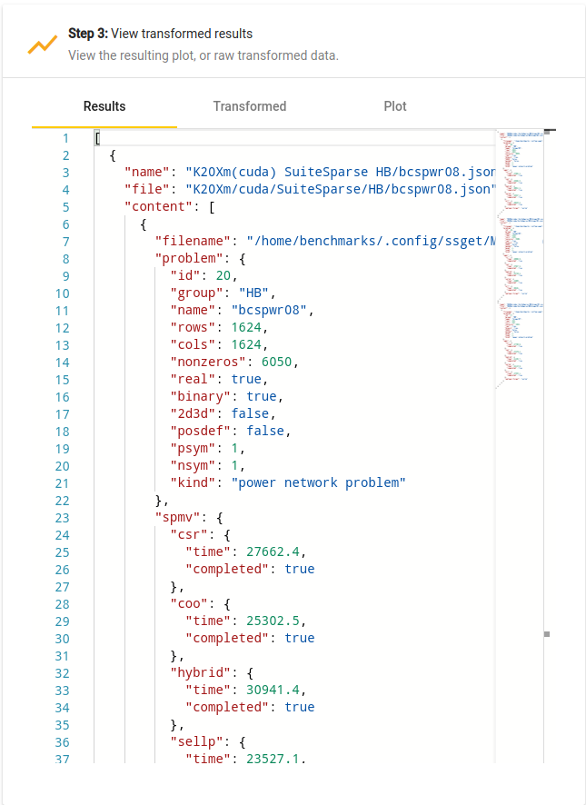Raw performance results viewer.

An example of raw data that is retrieved by GPE is shown in Figure [fig:raw-data]. All accessed result files are combined into one single JSON array of objects. Each object consist of properties such as the name and relative path to the result file, as well as its content.

Collecting useful insights from raw performance data is usually difficult, and distinct values need to be combined or aggregated before drawing conclusions. This is enabled by providing a script in the transformation script editor, marked with a green box on the left bottom in Figure [fig:web-app]. For example, the data in Figure [fig:raw-data] shows raw performance data of various sparse matrix-vector multiplication kernels (SpMV) on a set of matrices from the SuiteSparse matrix collection. It may be interesting to analyze how the performance of the CSR-based SpMV kernel depends on the average number of nonzeros per row. Neither of these quantities is available in the raw performance data. However, by following the tree of properties “content > problem > nonzeros”, “content > problem > rows” and “content > spmv > csr > time”, the total number of nonzeros in a matrix, the number of rows in a matrix, and the runtime of the CSR SpMV kernel can be derived. Since these are the only quantities needed to generate the comparison of interest, the transformation script editor can be used to write a suitable JSONata script [5] like so:

        content.{
            "sparsity": problem.(nonzeros / rows),
            "performance": 2 * problem.nonzeros /
                           spmv.csr.time
        }

The script is in real-time applied to the input data, and the result is immediately available in the “Transformed” tab of the data and plot viewer, as shown on Figure [fig:transformed-data].

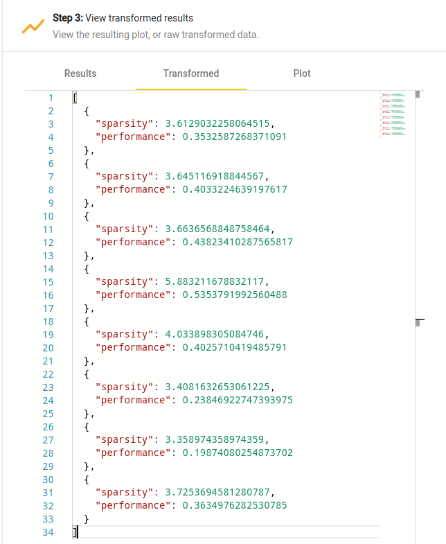Transformed data viewer.

The missing step is the visualization of the performance data. For that purpose, the data has to be transformed into a format that is readable for Chart.js, i.e. it has to be a Chart.js configuration object (as described in the Chart.js documentation[6]). Figure [lst:plot-script] provides a minimal extension of the script to generate a Chart.js configuration object. The visualized data is then available in the “Plot” tab of the data and plot viewer; see Figure [fig:plot].

        ($transformed := content.{
          "sparsity": problem.(nonzeros / rows),
          "performance": 2*problem.nonzeros /
                         spmv.csr.time
        }; {
          "type": "scatter",
          "data" : {
            "datasets": [{
              "label": "CSR",
              "data": $transformed.{
                "x": sparsity,
                "y": performance
              },
              "backgroundColor": "hsl(38,93%,54%)"
            }]
          }
        })

Plot generated by the example script given in Figure [lst:plot-script].

For first-time users, or to get a quick glance of the library’s performance, we provide a set of predefined JSONata scripts which can be used to obtain some performance visualizations without learning the language. These can be accessed from the “Select an example” dropdown menu of the transformation script editor. By default, the example scripts are retrieved from the Ginkgo performance data repository. However, the script location can be modified in the same way like the dataset location.

Examples

To conclude the presentation of GPE, we demonstrate its ability in analyzing performance data. The goal is not to analyze every aspect of the data in detail, but to show several (more complex) visualizations of a dataset, and the workflow to generate them. To that end, we look at the performance of Ginkgo’s SpMV kernels on the entire Suite Sparse matrix collection . Even though the whole dataset contains results for various architectures, we exclusively focus on the performance of Ginkgo’s CUDA executor on a K20Xm GPU. Thus, as a first step, the results are filtered to include only this architecture:

    $data := content[dataset.(
      system = "K20Xm" and executor = "cuda")]

In the following visualization examples we particularly focus on how to realize the data transformations needed to extract interesting data. The specific visualization configurations to generate appealing plots (including the labeling of the axes, the color selection, etc.), are well-documented and easy to integrate . The full JSONata scripts used to generate the graphs in this section are available as templates in the example script selector of GPE.

Fastest matrix format

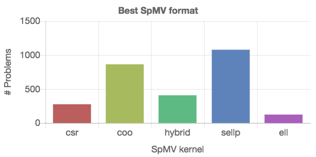
In a first example, we identify the “best” SpMV kernel by inspecting the number of problems for which that particular kernel is the fastest. To that end, we first extract the list of available kernels. Then, we split the list of matrices into sublists, where every sublist contains the matrices for which one of the kernels is the fastest. From this information, the numbers can be accumulated and arranged in a Chart.js configuration object. The JSONata script and the resulting plot are given in Figure [fig:best-format].

$formats := $data.spmv~>$keys(); $counts := $formats~>$map(function ($v) { $data.optimal[spmv = $v]~>$count() }); { "type": "bar", "data": { "labels": $formats, "datasets": [{ "data": $counts }] }, "options": { "scales": { "yAxes": [{ "ticks": { "beginAtZero": true } }]}} }

        $getColor := function($n, $id) {
          "hsl(" & $floor(360 * $id / $n)
                 & ",40%,55%)"
        };

        $formats := $data.spmv~>$keys();
        $plot_data := $formats~>$map(function($v, $i) {{
          "label": $v,
          "data": $data.{
            "x": problem.nonzeros,
            "y": 2 * problem.nonzeros /
                 (spmv~>$lookup($v)).time
          },
          "backgroundColor":
            $formats~>$count()~>$getColor($i)
        }});

        {
          "type": "scatter",
          "data": { "datasets": $plot_data },
          "options": { "scales": { "xAxes": [{
            "type": "logarithmic"
          }]}}
        }

A more detailed analysis

The results in Figure [fig:best-format] provide a summery, but no details about the generality of the kernels. Each kernel “wins” for a portion of matrices, but it is impossible to say which kernel to choose for a specific matrix. Since the SpMV kernel performance usually depends on the number of nonzeros in the matrix, we next visualize the performance of the distinct SpMV kernels depending on the nonzero count. From the technical point of view, different SpMV kernels have to be identified in the set, and the relevant data has to be extracted from the dataset as shown on the left side in Figure [fig:nonzeros-performance].

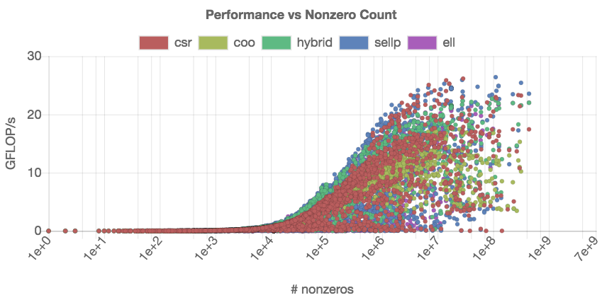
To distinguish the performance of the distinct SpMV kernels data in the scatter plot, we encode the kernels using different colors. This is realized via a script that defines a helper $getColor function which selects a set of color codes that are equally-distant in the color wheel.

Figure [fig:nonzeros-performance] reveals more details about the performance of the distinct SpMV kernels. Inside the GPE application, the points representing distinct kernels can be activated and deactivated by clicking on the appropriate label in the legend. We note that this plot contains about 15,000 individual data points ( > 3, 000 test matrices, 5 SpMV kernels), which makes the interactive analysis very resource-demanding.

Comparison of CSR and COO formats

From comparing the performance of the CSR and the COO kernel in Figure [fig:nonzeros-performance], we conclude that the CSR format achieves better peak performance than COO. However, the COO performance seems more consistent as (for large enough matrices), it never drops below 5 GFLOP/s. This suggest that there exist matrices for which the CSR kernel is not suitable. We may assume that load balancing plays a role, and the regularity of matrices having a strong impact on the performance of the CSR kernel. Indeed, the CSR kernel distributes the matrix rows to the distinct threads, which can result in significant load imbalance for irregular matrices. The COO kernel efficiently adapts to irregular sparsity patterns by balancing the nonzeros among the threads .

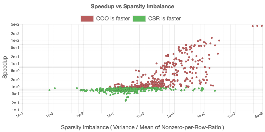
To analyze this aspect, we create a scatter plot that relates the speedup of COO over CSR to the “sparsity imbalance of the matrices.” We derive this metric as the ratio between the standard deviation and the arithmetic mean of the nonzero-per-row distribution. We expect to see a slowdown (speedup smaller than one) for problems with low irregularity, and a speedup (larger than one) for problems with higher irregularity. The previous analysis in Figure [fig:nonzeros-performance] included problems that are too small to generate useful performance data. In response, we restrict the analysis to problems containing at least 100, 000 nonzeros. The script for realizing the performance comparison and the resulting graph indicating the validity of the assumption are given in Figure [fig:csr-coo-speedup].

$plot_data := $data[problem.nonzeros > 100000].{ "x": problem.row_distribution.( $sqrt(variance) / median), "y": spmv.(csr.time / coo.time) }; { "type": "scatter", "data": { "datasets": [{ "label": "COO is faster", "data": $plot_data[y >= 1], "backgroundColor": "hsl(0,40%,55%)" }, { "label": "CSR is faster", "data": $plot_data[y < 1], "backgroundColor": "hsl(120,40%,55%)" }]}, "options": { "scales": { "xAxes": [{ "type": "logarithmic" }], "yAxes": [{ "type": "logarithmic" }] }} }

[1]: The authors would like to thank the BSSw and the xSDK community efforts, in particular Mike Heroux and Lois Curfman McInnes, for promoting guidelines for a healthy software life cycle.