Explained machine learning models and projects based on ML
Basic machine learning algorithms:
1.Linear regression
2.Logistic regression
3.Support Vector Machines
4.Naive Bayes
(below coming soon...)
5.Decision trees
6.Random Forest
7.k- Means clustering
8.k-Nearest neighbors
Linear regression is very simple and basic.First, linear regression is supervised model, which means data should be labelled.Linear regression will find the relationships between features(x1,x2,x3....), which represent as coefficients of these variables.
Let's look at a simple linear regression equation:
▷ θ1 is the coefficient of the independent variable (slope)

▷ θ0 is the constant term or the y intercept.
Then consider this dataset as tuples of (1, 18), (2, 22), (3, 45), (4, 49), (5, 86)
• We might want to fit a straight line to the given data

• Assume to fit a line with the equation Y = θ1X + θ0

• Our goal is to minimize errors
To minimize the amount of distance(errors), we need to find proper θ1 and θ0.We build a function ,which often referred to as a lost function,.
lost function has three common formula:
    (1)MSE(Mean Squared Error)
    (2)RMSE(Root Mean Squared Error)
    (3)Logloss(Cross Entorpy loss)
In this case, we choose Mean Squared Error.
So when we want to fit a line to given data, we need to minimize the lost function.
then, computing lost function:
Since cost function is a ”Convex” function, when its derivative is 0, the cost function hits bottom. So loss minimized at θ = 14.96.
Now we have a polynomial linear regression, suppose each entity x has d dimensions:
Similarly, we get the lost function :
So in order to minimize the cost function, we need to choose each θi to minimize l(θ0,θ1...),this is what we called Gradient Descent.
Gradient Descent is an iterative algorithm,Start from an initial guess and try to incrementally improve current solution,and at iteration step θ(iter) is the current guess for θi.
Suppose ▽l(θ) is a vector whose ith entry is ith partial derivative evaluated at θi
In privious sessions, we got the loss function, which is
then do expansion:
Since it has mutiple dimensions,we compute partial derivatives:
Now we can compute components of the gradients and then sum them up and update weights in the next iteration.

• Here λ is the ”learning rate” and controls speed of convergence
• ▽l(θ iter) is the gradient of L evaluated at iteration ”iter” with parameter of qiter
• Stop conditions can be different
When to stop
  Stop condition can be different, for example:
    • Maximum number of iteration is reached (iter < MaxIteration)
    • Gradient ▽l(θ iter ) or parameters are not changing (||θ(iter+1) - θ(iter)|| < precisionValue)
    • Cost is not decreasing (||l(θ(iter+1)) - L(θ(iter))|| < precisionValue)
    • Combination of the above
more detailed pseudocode to compute gradient:
// initialize parameters
iteration = 0
learning Rate = 0.01
numIteration = X
theta = np.random.normal(0, 0.1, d)

while iteration < maxNumIteration:

  calculate gradients
  //update parameters
  theta -= learning Rate*gradients
  iteration+=1
Check here
We will always face over-fitting issue in real problem. over-fitting issue is that the parameters of model are large and model's rebustness is poor, which means a little change of test data may cause a huge difference in result.So in order to aviod over-fitting,
We need to remove parameters which have little contribution and generate sparse matrix, that is, the l1 norm( mean absolute error):
where l is lost function, ∑ i|θi| is l1 regularizers, λ is regularization coefficient, θi is parameters.
we can visualize l1 lost function:
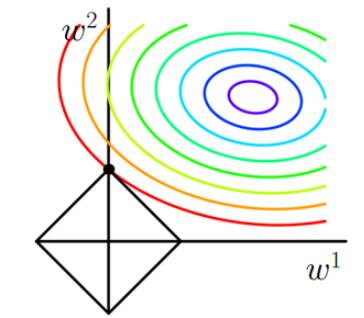
The contour line in the figure is that of l, and the black square is the graph of L1 function. The place where the contour line of l intersects the graph of L1 for the first time is the optimal solution. It is easy to find that the black square must intersect the contour line at the vertex of the square first. l is much more likely to contact those angles than it is to contact any other part. Some dimensions of these points are 0 which will make some features equal to 0 and generate a sparse matrix, which can then be used for feature selection.
We can make parameters as little as possible by implement l2 norm:
where l is lost function, ∑ i|θi|² is l2 regularizers, λ is regularization coefficient, θi is parameters.
we can visualize l2 lost function:
In comparison with the iterative formula without adding L2 regularization, parameters are multiplied by a factor less than 1 in each iteration, which makes parameters decrease continuously. Therefore, in general, parameters decreasing continuously.
Logistic regression is supervised model especially for prediction problem.It has binary-class lr and multi-class lr.
Suppose we have a prediction problem.It is natural to assume that output y (0/1) given the independent variable(s) X ,which has d dimensions and model parameter θ is sampled from the exponential family.
It makes sense to assume that the x is sampled from a Bernoulli and here is the log-likelihood:
Given a bunch of data for example,suppose output Y has (0/1):
(92, 12), (23, 67), (67, 92), (98, 78), (18, 45), (6, 100)

Final Result in class: 0, 0, 1, 1, 0, 0

• If coefs are (-1, -1), LLH is -698
• If coefs are (1, -1), LLH is -133
• If coefs are (-1, 1), LLH is 7.4
• If coefs are (1, 1), LLH is 394
However this is not enough to get the loss function, logistic regreesion needs a sigmoid function to show the probability of y = 0/1,which is :
The parameter ω is related to X that is, assuming X is vector-valued and ω can be represent as :
where θ is regression coefficent and j is entity's jth dimension .
Now its time to implement Log-likelihood in logistic regression, written as:
Now calculate loss function.As gradient descent need to minimize loss function,the loss function should be negative LLH:
Appling regularization (l2 norm):
where j is entity's jth dimension.
Suppose θj is jth partial derivative :
Since it has mutiple dimensions,we compute partial derivatives:

Check here
In binary-class lr model, we use sigmoid function to map samples to (0,1),but in more cases, we need multi-class classfication, so we use softmax function to map samples to multiple (0,1).
Softmax can be written as a hypothesis function :
where k is the total number of classes, i is ith entity.
then we can get the loss function,which is also be called log-likelihood cost:
where 1{expression} is a function that if expression in {} is true then 1{expression} = 1 ,else 0.
then rearrange it, and add l2 norm :
Suppose θj is jth partial derivative :
Check here
Traditional svm is binary-class svm, and there is also multi-class svm.
Suppose there is a dataset that is linearly separable, it is possible to put a strip between two classes.The points that keep strip from expending are 'support vector'.
So basiclly, all points x in any line or plane or hyperplane can be discribed as a vevtor with distance b:
Now here is a point x and we need to caluculate the distance (which can be discribed as y) between this point and plane:
Notice y should be -1 or 1 to determine which of the sides the point x is.
This is because in basic svm, it choose two planes:
where y > 1 then x is '+'(or x is positive sample)
where y < -1 then x is '-'(or x is negative sample)
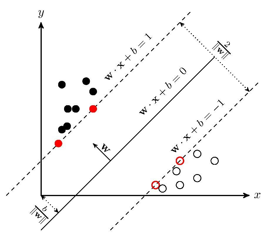
The distance between two planes are ,so we need to maximize this distance to get optimal solution.
First, define a normal loss function:
when this loss function is hinge loss, it is exactly svm's loss function:
then add l2 norm, the final loss function is :
We can use Chain rule to compute the derivative:
then calculate derivatives for two parts:
In conclusion, the final gradient is :
(1)if :
below fomula(1) = 0, which means the derivative =
(2)if :
below fomula(1) = , which means the derivative =
then the final derivatives for batch of data can be written as:
Check here
Different from binary-class svm, multi-class svm's loss function requires the score on the correct class always be Δ(a boundary value) higher than scores on incorrect classes.
Suppose there is a dataset, the ith entity xi contains its features(has d features represent as vector) and class yi, then given svm model f(xi,w) to calculate the scores(as vector) in all classes,here we use si to represent this vector.
According to the definition of multi-class svm, we can get ith entity xi's loss fucntion:
For example:
Suppose there are 3 classes, for the ith sample xi, we get scores = [12,-7,10],where the first class(yi) is correct.Then we make Δ=9, applying the below loss function, we can calculate the loss of xi:
As w is a vector in loss function, we expend loss function:
Then add l2 norm:
As yi and j are different, we calculate wyi's derivative for ith entity xi first:
then calculate wj's derivative for ith entity xi:
The gradient of vector wi contians wj(from 1 to d) and each wj's value depends on the value of :
So the gradient for batch of data can be written as:
Check here
Naive Bayes is based on Bayes' theorem, which is :
we suppose dataset has m entities, each entitiy has n dimensions.There are k classes, define as :
We can get p(X,Y)'s joint probability via Bayes' theorem:
Suppose n dimensions in entity are independent of each other :
Notice some dimentions are discrete type,while others are continuous type,
suppose Sck is subset where item's class is Ck, S k,xi is subset of Sk where item's i dimension is xi.
discrete type
continuous type
Suppose Sk,xi are subject to Gaussian distribution:
then we can get:
After comparing p(X,Y) in all classes, we can get the result class which has the highest p(X,Y).
For example, if there is no sample(which belongs to Ck and ith dimension is Xa), then .
Becasue of the continued product,
use laplacian correction:
where |Sck| is the number of subset Sck(where items are class ck) , |S| is number of whole dataset, N is the number of classes
where |S k,xi| is the number of the subset of Sck where item's i dimension is xi, Ni is the number of possible value of ith attribute.
MultinomialNB is naive Bayes with a priori Gaussian distribution, multinomialNB is naive Bayes with a priori multinomial distribution and BernoullinB is naive Bayes with a priori Bernoulli distribution.
These three classes are applicable to different classification scenarios. In general, if the distribution of sample features is mostly continuous values, Gaussiannb is better. MultinomialNb is appropriate if the most of the sample features are multivariate discrete values. If the sample features are binary discrete values or very sparse multivariate discrete values, Bernoullinb should be used.
Variations of Gradient Descent depends on size of data that be used in each iteration:
  • Full Batch Gradient Descent (Using the whole data set (size n))
  • Stochastic Gradient Descent (SGD) (Using one sample per iteration (size 1))
  • Mini Batch Gradient Descent (Using a mini batch of data (size m < n))
BGD has a disadvantage: In each iteration, as it calculates gradients from whole dataset, this process will take lots of time.BGD can't overcome local minimum problem, because we can not add new data to trainning dataset.In other word, when function comes to local minimum point, full batch gradient will be 0, which means optimization process will stop.
SGD is always used in online situation for its speed.But since SGD uses only one sample in each iteration, the gradient can be affacted by noisy point, causeing a fact that function may not converge to optimal solution.
MSGD finds a trade-off between SGD and BGD.Different from BGD and SGD, MSGD only pick a small batch-size of data in each iteration, which not only minimized the impact from noisy point, but also reduced trainning time and increased the accuracy.
The learning rate is a vital parameter in gradient descent as learning rate is responsible for convergence, if lr is small, convergent speed will be slow, on the contrary,when lr is large, function will converge very fast.
compare different learning rate:

So how to find a proper learning rate? If we set lr a large value, the function will converge very fast at beginning but may miss the optimal solution,but if we set a small value, it will cost too much time to converge. As iterations going on, we hope that learning rate becomes smaller.Because when function close to optimal solution, the changing step should be small to find best solution.So we need to gradually change learning rate.
Here is a very simple method, which name is Bold Driver to change learning rate dynamicly:
At each iteration, compute the cost l(θ0,θ1...)
Better than last time?
If cost decreases, increase learning rate l = 1.05 * l
Worse than last time?
l = 0.5 * l If cost increases, decrease rate
A better method is Time-Based Decay .The mathematical form of time-based decay is lr = lr0/(1+kt)
where lr, k are hyperparameters and t is the iteration number.
Those graphs illustrate the advantages of Time-Based Decay lr vs constant lr:
constant lr
Time-Based Decay lr
Also, we know that the weights for each coefficent is different, which means gradients of some coefficents are large while some are little.So in traditional SGD, changes of coefficents are not synchronous.So we need to balance the coefficents when doing gradient descent.
To deal with this issue, we can use SGDM, Adagrad(adaptive gradient algorithm), RMSProp, Adam
SGDM is SGD with momentum.It implement momentum to gradient:
where m0 = 0, λ is momentum's coefficent, η is learing rate.
visualization:

Adagrad will give each coefficent a proper learning rate:
θ : coefficents

∂l/∂θ : gradient

η: learning rate

hj: sum of squares of all the previous θj's gradients
when updating coefficent, we can adjust the scale by mutiplying 1/√h.
But as iteration going on, h will be very large, making updating step becomes very small.
RMSProp can optimize this problem.RMSProp uses an exponential weighted average to eliminate swings in gradient descent: a larger derivative of a dimension means a larger exponential weighted average, and a smaller derivative means a smaller exponential weighted average. This ensures that the derivatives of each dimension are of the same order of magnitude, thus reducing swings:
√hj can be 0 some times, so we add a small value c to √hj
RMSProp code here
def RMSprop(x, y, lr=0.01, iter_count=500, batch_size=4, beta=0.9):
    length, features = x.shape
    data = np.column_stack((x, np.ones((length, 1))))
    w = np.zeros((features + 1, 1))
    h, eta = 0, 10e-7
    start, end = 0, batch_size
    for i in range(iter_count):
        # calculate gradient
        dw = np.sum((np.dot(data[start:end], w) - y[start:end]) * data[start:end], axis=0) / length
        # calculate sum of square of gradients
        h = beta * h + (1 - beta) * np.dot(dw, dw)
        # update w
        w = w - (lr / np.sqrt(eta + h)) * dw.reshape((features + 1, 1))

        start = (start + batch_size) % length
        if start > length:
            start -= length
        end = (end + batch_size) % length
        if end > length:
            end -= length
    return w
Adam is another powerful optimizer.It not only saved the sum of square of history gradients(h) but also save sum of history gradients(m, known as momentum):
If m and h are initialized to the 0 vectors, they are biased to 0, so bias correction is done to offset these biases by calculating the bias corrected m and h:
t means t th iteration.
Adam code here
def Adam(x, y, lr=0.01, iter_count=500, batch_size=4, beta1=0.9,beta2 = 0.999):
    length, features = x.shape
    data = np.column_stack((x, np.ones((length, 1))))
    w = np.zeros((features + 1, 1))
    m, h,eta = 0, 0,10e-7
    start, end = 0, batch_size
    for i in range(iter_count):
        # calculate gradient
        dw = np.sum((np.dot(data[start:end], w) - y[start:end]) * data[start:end], axis=0) / length
        # calculate sums
        m = beta1 * m + (1 - beta1) * dw
	h = beta2 * h + (1 - beta2) * np.dot(dw, dw)
	# bias correction
	m = m/(1- beta1)
	h = h/(1- beta2)
        # update w
        w = w - (lr / np.sqrt(eta + h)) * m.reshape((features + 1, 1))

        start = (start + batch_size) % length
        if start > length:
            start -= length
        end = (end + batch_size) % length
        if end > length:
            end -= length
    return w
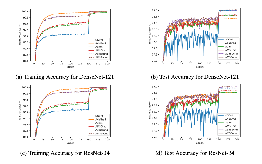
By far, the most popular models are SGDM and Adam.

This graph illustrates that SGDM is always used in computer vision whereas Adam are popular in NLP.
For Adam, there are SWATS,AMSGrad,AdaBound,and AdamW.
For SGDM, there are SGDMW,SGDNM
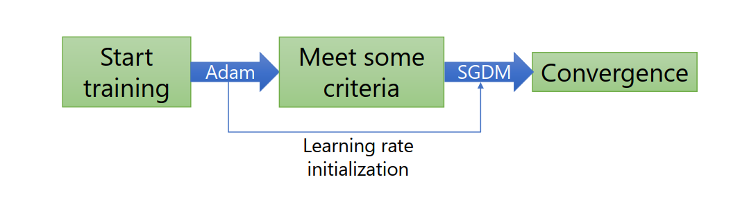
combine Adam and SGDM:
optimize Adam in changing the way to update hj:
AMSGrad makes learning rate monotone decrease and waives small gradients.
AdaBound limits learning rate in a certain scale:
Add weight decay to Adam:
Add weight decay to SGDM:
where m0 = 0, λ is momentum's coefficent, η is learing rate, γ is weight decay coefficent.
SGDMN(SGDM with Nesterov) is aimed to solve local optimal problem.When local optimal problem happend, SGDMN will do an additional calculation to determine whether to stop iteration:
Nadam(Adam with Nesterov) is aimed to solve local optimal problem.When local optimal problem happend, NAdam will do an additional calculation to determine whether to stop iteration:
comparation between these optimizers ,lets see the differenes of those optimizers:
kaggel link :
https://www.kaggle.com/uciml/mushroom-classification
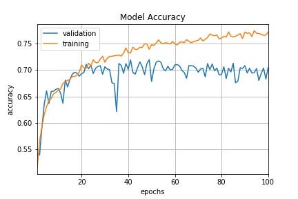
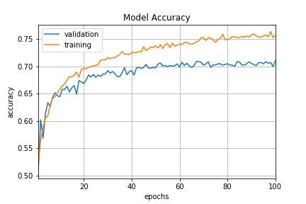
This project is mushroom classification. There are about 2 categories (edible or poisonous) and 8124 records (52% edible and 48% poisonous). For this project, I have tried three machine learning models: SVM , Random forest and logistic regression. All three models have good performances: Compare recall, precision, f1-score for both class F1_score > 95% Accuracy > 95%
This dataset includes descriptions of hypothetical samples corresponding to 23 species of gilled mushrooms in the Agaricus and Lepiota Family Mushroom drawn from The Audubon Society Field Guide to North American Mushrooms (1981). Each species is identified as definitely edible, definitely poisonous, or of unknown edibility and not recommended. This latter class was combined with the poisonous one. The Guide clearly states that there is no simple rule for determining the edibility of a mushroom; no rule like "leaflets three, let it be'' for Poisonous Oak and Ivy.
Code