2. User Guide
This page walks you through on how to use Model Explorer.
Table of Contents
- Select models
- Visualization UI Overview
- Model graph and side panel
- Toolbar
- Handle multiple models
- Custom node data
- Misc
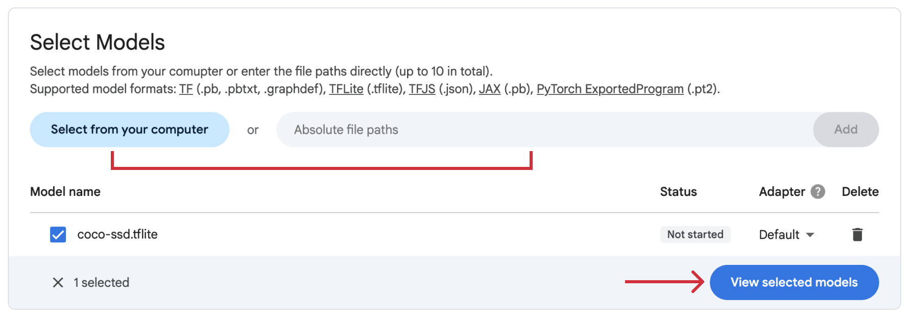
In the home page, select models to visualize by clicking the "Select from your computer" button, or by entering the absolute model paths (separated by comma) in the text box. You can also drag-and-drop model files onto the home page.
Once you've selected your models, click the "View selected models" button. Model Explorer will process your files and take you to the visualization page.
Tip
For faster processing of large models, enter the file path directly instead of using the "select from your computer" button. This avoids the overhead of copying the file to a temporary directory.
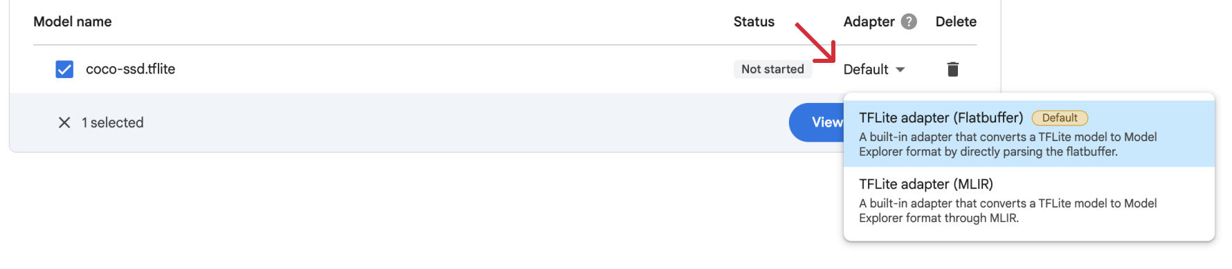
Model Explorer uses "adapters" to transform your model files into an intermediate format that Model Explorer can understand and visualize. The "default" adapter should handle most common use cases. To pick a different adapter, click the adapter drop down menu for a specific model.
To visualize a PyTorch model, the corresponding module has to be exported to an ExportedProgram by using torch.export and save the file with the pt2 file extension. See the official doc for instructions.
Note
torch.export is under active development and the exported graph using a older version of PyTorch might not work in newer versions. To ensure compatibility, make sure to use the same version of torch installed by ai-edge-model-explorer. Alternatively, use the API in your Python program to directly visualize a PyTorch module.
Once the model has been loaded and processed successfully, it will be displayed starting from its root layer in the main visualization UI. The UI has the following components:
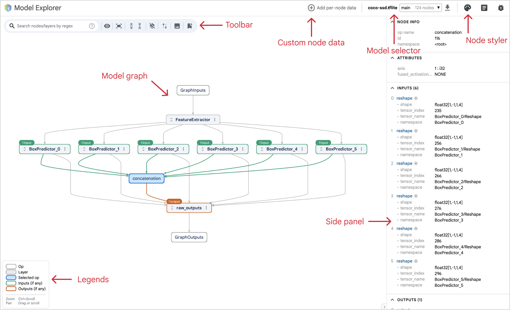
Sub-sections below will provide detailed explanation for each component.
-
Zoom
Ctrl + scroll up/down, or pinch on touchpad. -
Zoom in to an area
Ctrl or ⌘ (Mac) + mouse drag to drag out an area to zoom in to. -
Pan
Drag the graph, scroll the mouse wheel, or pan on the touchpad. -
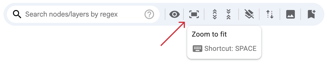
Fit to screen
Press theSPACEkey, or click on the "Fit to screen" button on the toolbar.
Tip
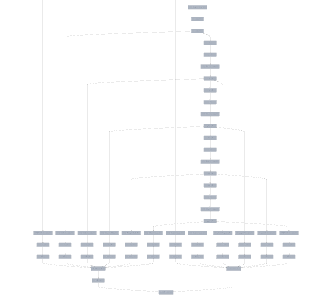
To maintain readability when zoomed out, Model Explorer automatically renders op nodes as color blocks, making it easier to understand your model's structure. An example:
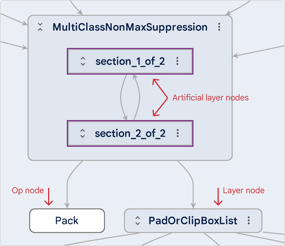
There are three types of nodes in Model Explorer:
-
Op nodes
They have white background. An op node does not have children. -
Layer nodes
They have light-blue background colors with action icons. A layer node can have other layer nodes and/or op nodes as its children. -
Artificial layer nodes
To improve layout latency and readability for large graphs/layers, Model Explorer will automatically partition the large graphs into artificial layers/sections by walking through the graph from roots in a depth-first-search order, ensuring that each section contains no more than a threshold (1000 children by default). These artificial layers will be rendered with a purple border to distinguish them from regular layers.
Tip
You can change the threshold of artificial layer node count in settings.
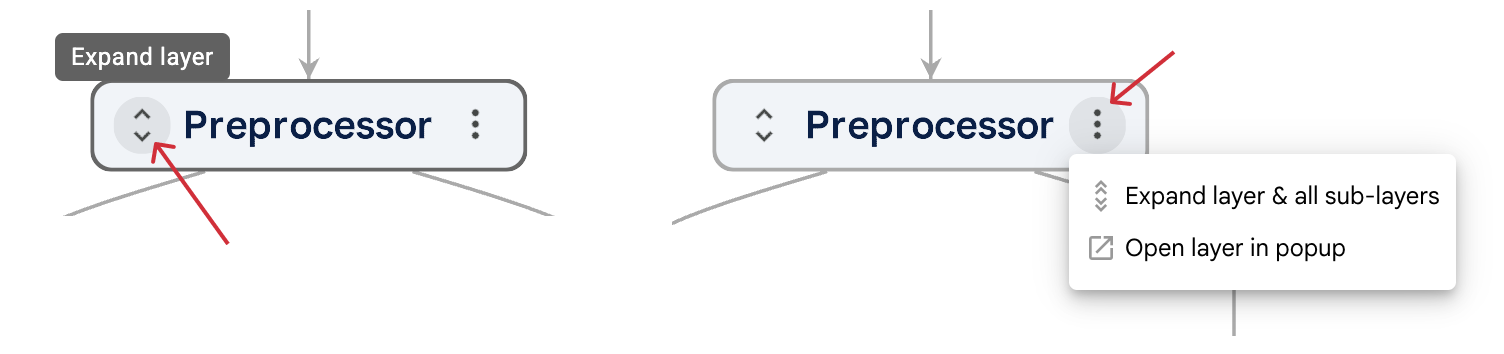
To reveal the content of a layer, Click the ![]() "expand" icon, or double-click the layer node. To collapse an expanded layer, click the
"expand" icon, or double-click the layer node. To collapse an expanded layer, click the ![]() "collapse" icon, or double-click the layer node.
"collapse" icon, or double-click the layer node.
To recursively expand all layers under a layer, open the overflow menu on a layer node and select "expand layer and all sub-layers".
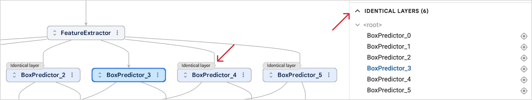
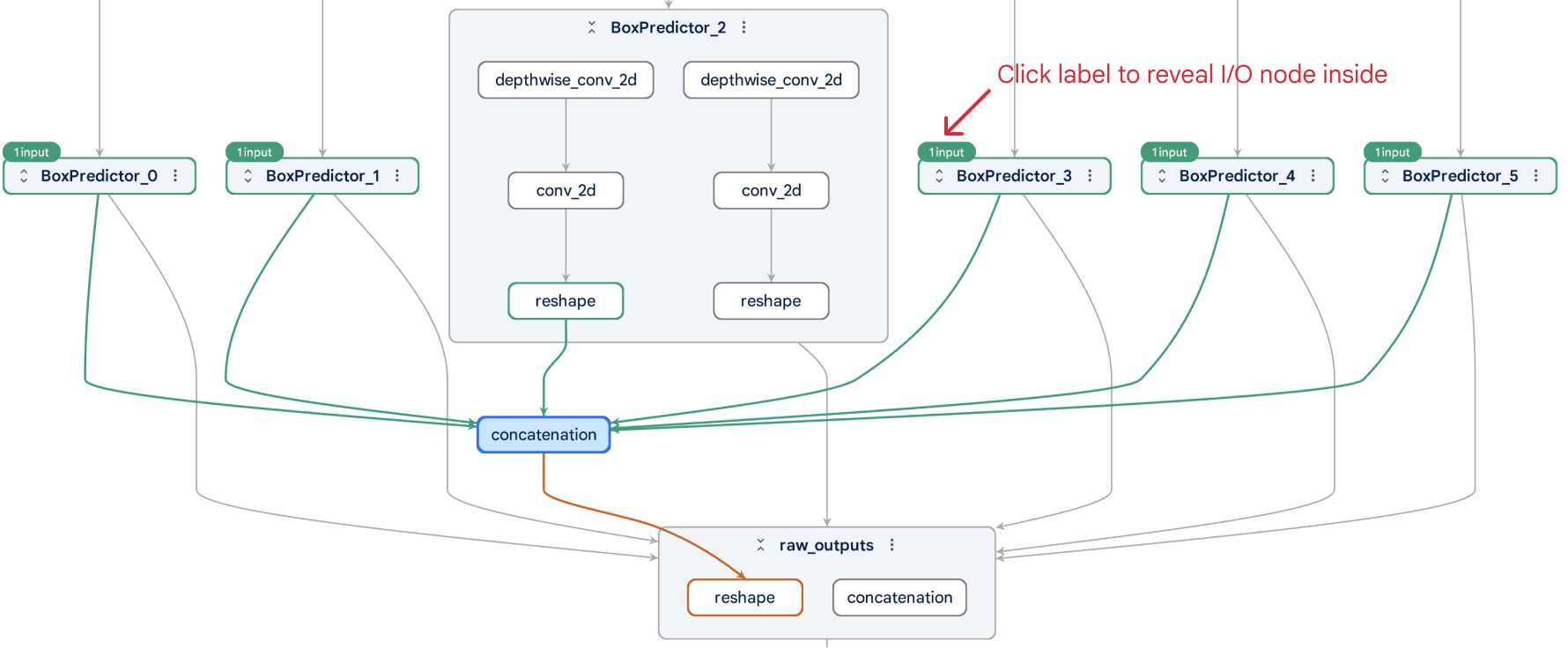
When a layer node is selected, Model Explorer will automatically highlight identical layers (in terms of descendant nodes and their connections inside the layer) with light blue color and a label. It will also show the list of identical layers in the side panel.
In the following screenshot, after user selects the BoxPredictor_3 layer, it shows that it is identical to other 4 box predictor layers.
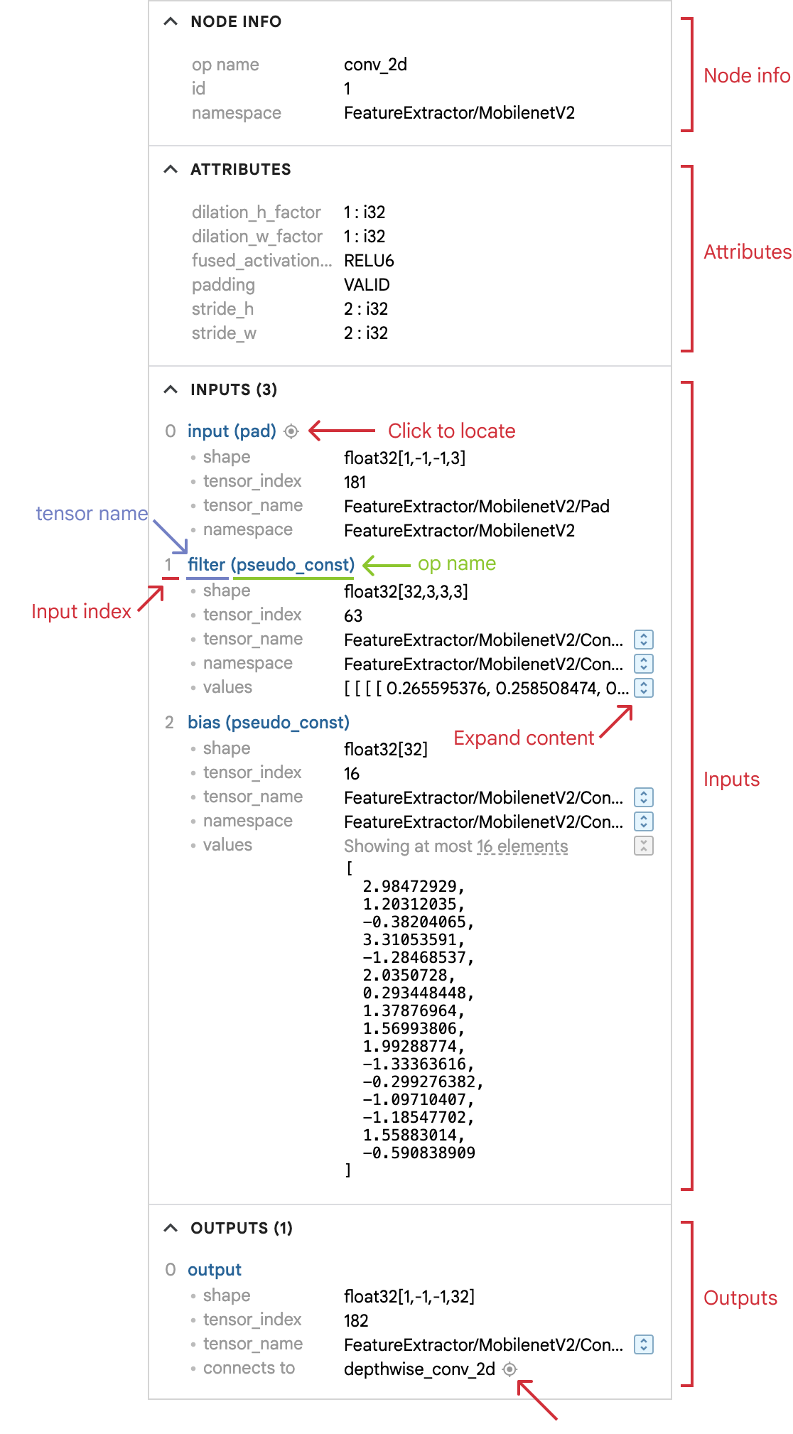
When an Op node is selected, its basic info, attributes, inputs, and outputs are displayed in the side panel. Its input and output nodes will also be highlighted in the model graph.
The side panel offers insights into your selected op. Click the ![]() icon to expand the value content when it overflows.
icon to expand the value content when it overflows.
-
Node info
Basic info of the node, such as id, namespace (which layer the node is located), etc. -
Attributes
The attributes (key/value paris) of the node. -
Inputs
The selected op's input tensors with key tensor metadata, such as tensor name and shape. Clicking the op name of an input tensor (indicated by a "locator" icon) will scroll the graph directly to that node's position and expand all its ancestor layers to reveal the node.
 -
Outputs
The selected op's output tensors, their metadata, and the ops they connect to. Clicking the name of a connected op node will locate that op node in the graph.
Tip
Using Alt+Click on a node row will locate and select the node.
In the model graph, the selected node and its input and output nodes/edges are highlighted with different colors:
- Blue: selected node.
- Green: input nodes and edges.
- Red: output nodes and edges.
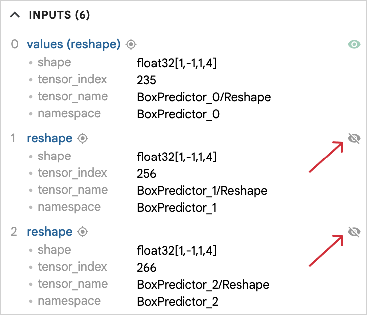
If an input/output node is in a collapsed layer, a label with the number of input/output nodes inside will appear on the corresponding layer node. Clicking the label will expand the layer and automatically locate the input/output node inside. If there are multiple input/output nodes, a menu will appear to let you select which node to locate.
Clicking the "eye" icon next to each input or output will toggle the visibility of its highlight in the model graph.
Tip
Use Alt+Click to highlight a single input/output and hide the rest.
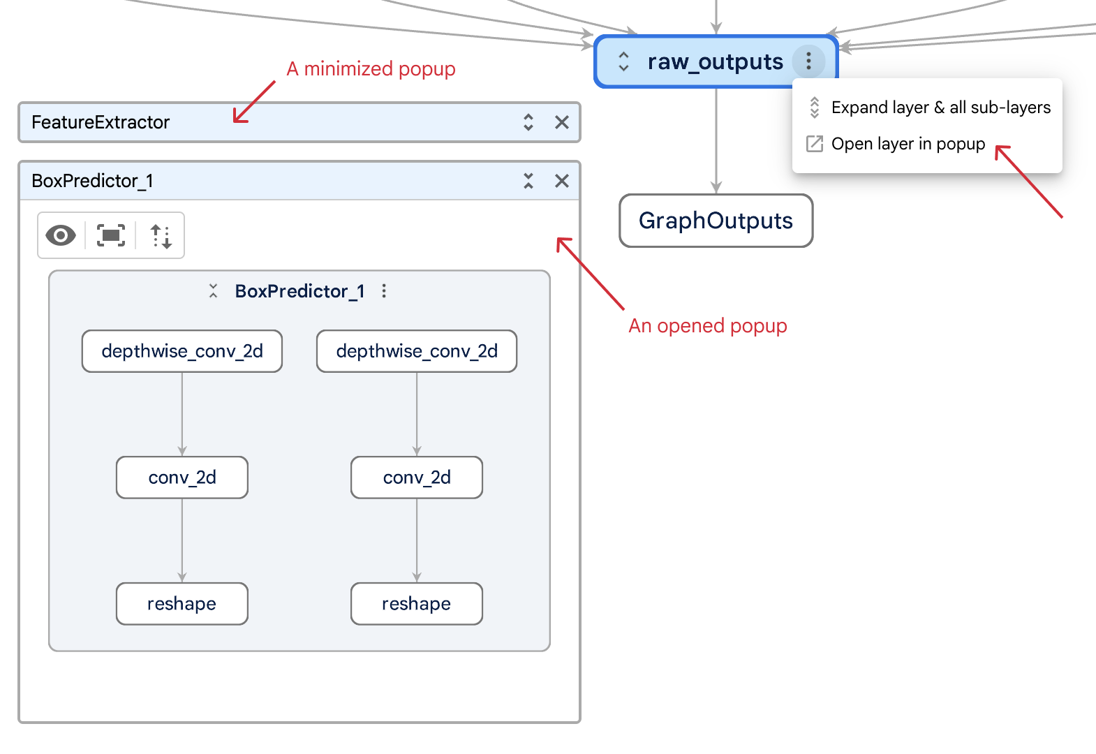
You can open a layer in a movable popup panel by selecting "Open layer in popup" item in a layer node's overflow menu. The selected layer will become the root of the graph in the popup, and you can navigate the graph in the panel the same way as in the main graph. The popup panel can also be moved, resized, and minimized, and you can open multiple popup panels rooted at different layers.
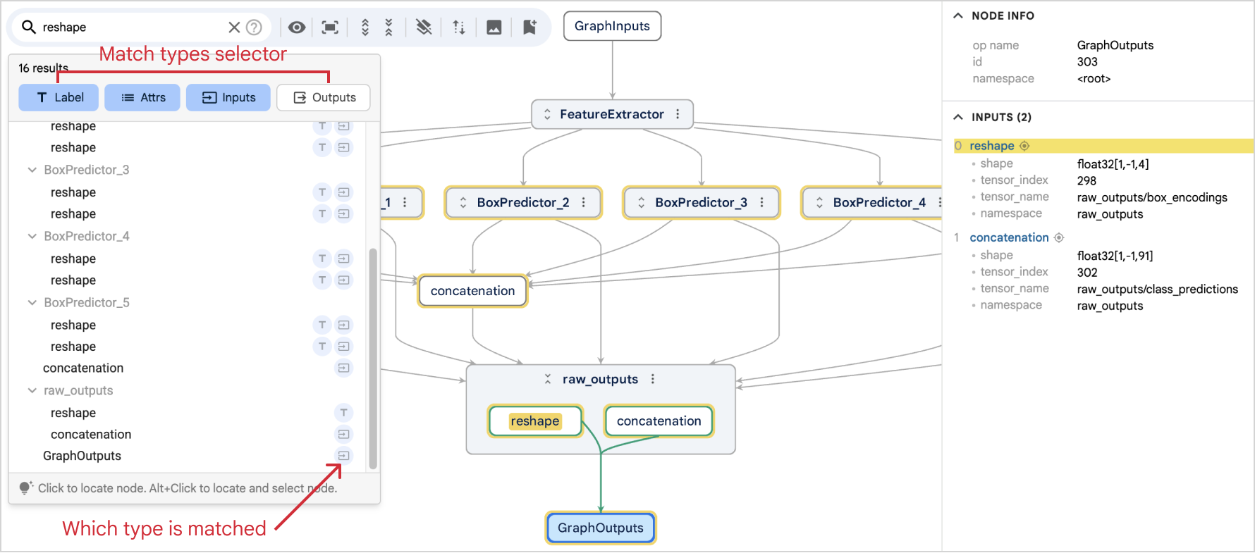
You can use regex to search for nodes based on 4 match types: ![]() label,
label, ![]() attributes,
attributes, ![]() inputs, and
inputs, and ![]() outputs.
outputs.
-
Label
The entered regex will try to match the labels being displayed on nodes. -
Attributes
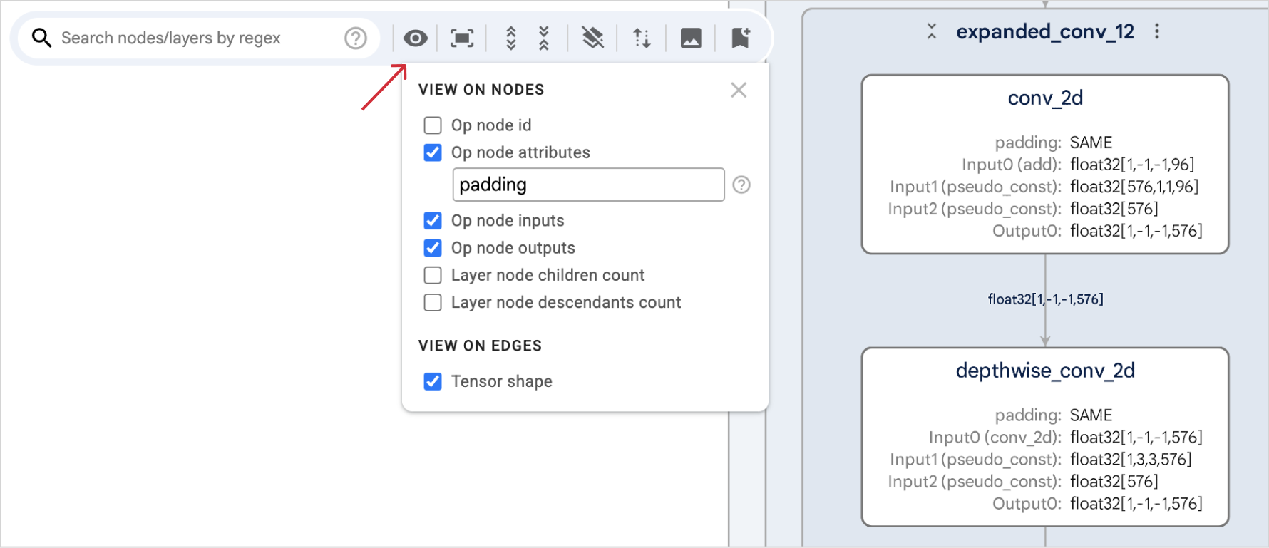
The entered regex will try to match the string{attr_key}={attr_value}or{attr_key}:{attr_value}for each attribute in a node. For example, assume node A has an attributepadding: SAME, and node B has an attributepadding: VALID. Then:- The regex
padding=will match both nodes. - The regex
padding:[SAME|VALID]will match both nodes too. - The regex
SAMEwill only mach node A.
- The regex
-
Inputs
The entered regex will try to match the label and the tensor's metadata of a node's input nodes. When matching tensor metadata, it will try to match the string{metadata_key}={metadata_value}or{metadata_key}:{metadata_value}. For example, a regexshape=.*x3will match a node with input metadatashape: 1x64x64x3. -
Outputs
The entered regex will try to match the label and the tensor's metadata of a node's output nodes.
The results will be shown below the search box organized by their location within the graph hierarchy. Each item in the list shows the node label as well as which "match type" of it got matched. Clicking an item will locate the node in the graph. The matching nodes and the part that got matches will be highlighted in the model graph and the side panel.
In the following screenshot, user is searching for "reshape", and the "GraphOutputs" node is a match because one of its inputs is connected to a "reshape" node.
Note
We're working on supporting multiple search queries for better results filtering. Stay tuned!
Use the "View on nodes/edges" button on the toolbar to choose which information you want to be displayed directly on your model graph. Each time you make a selection under the "View on node" section, the graph will automatically re-layout due to node size changes. For node attributes, you can enter a filter (regex) to specify which attribute to show. For node inputs, node outputs, and edge labels, Model Explorer currently only supports showing shapes.
Tip
You can change the font size of edge labels in settings.
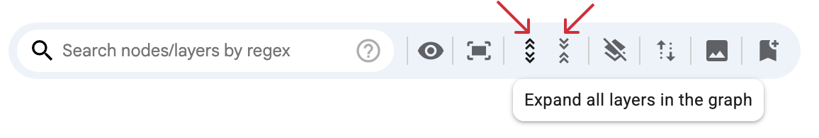
Use the buttons shown below on the toolbar to expand/collapse all the layers (including nested layers) in the graph. Expanding all layers might take some time for large graphs.
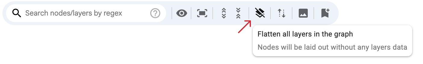
Sometimes, the detailed layer structure within a model graph can add visual complexity. If you need a more streamlined view, Model Explorer allows you to flatten all layers. This removes layer groupings, rearranges nodes accordingly, and can help you focus on the core node-to-node connections.
Click the button below to toggle it on/off.
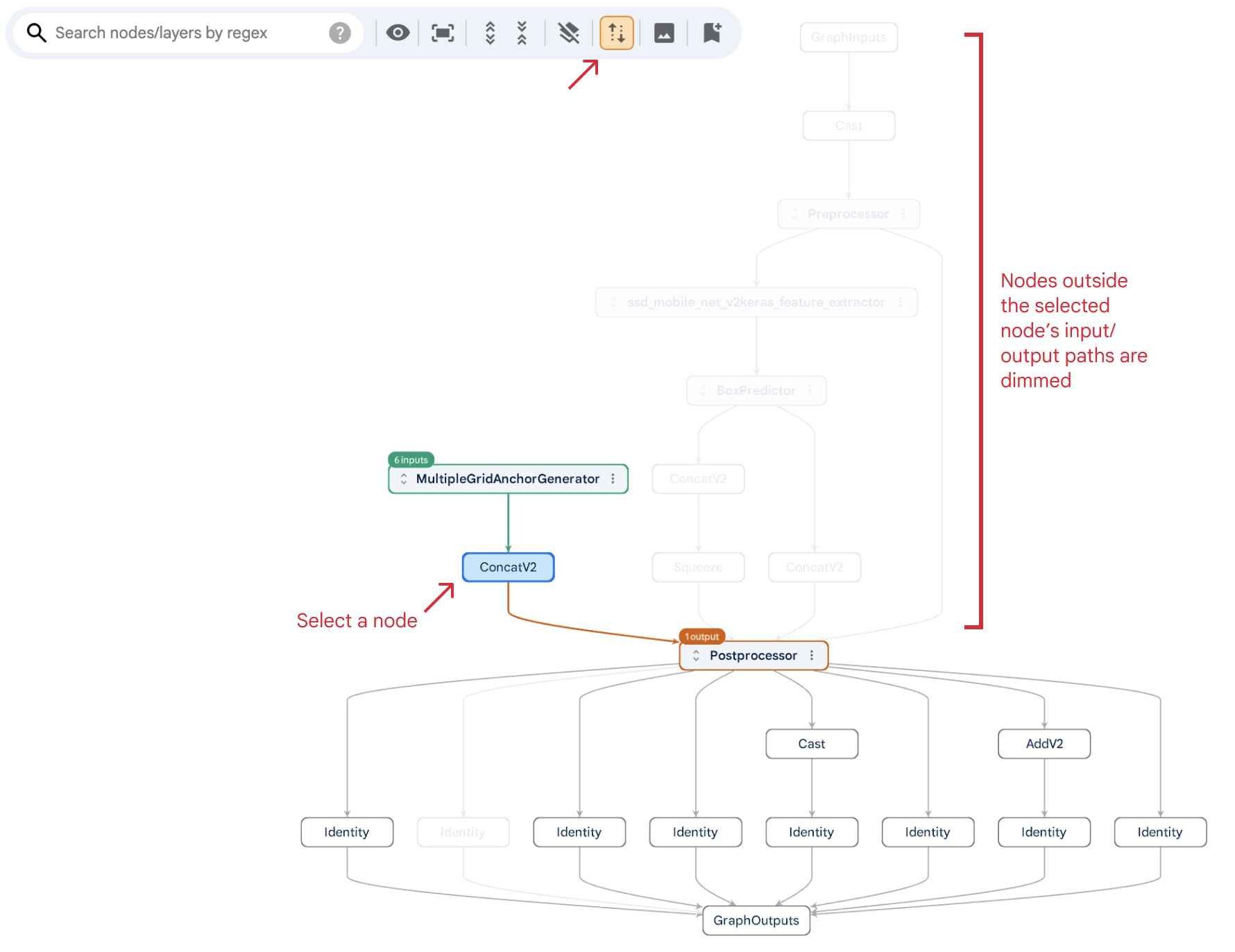
Toggle on the "trace inputs and outputs" button on the toolbar as shown below and Model Explorer will highlight the selected op node's ancestors and descendants nodes and dim the rest.
Click the button below to download the model graph as a PNG file. You can select whether to download the graph clipped to the current viewport, or the whole graph. Note that the maximum size of the generated PNG file is 5000px x 5000px.

You can use the bookmark button on the toolbar shown below to save the current state of the graph. The state includes:
- The selected node
- Expanded/collapsed layers
- Zoom level and pan position
- The selected items to overlay on nodes/edges
- Whether the layers are flattened or not
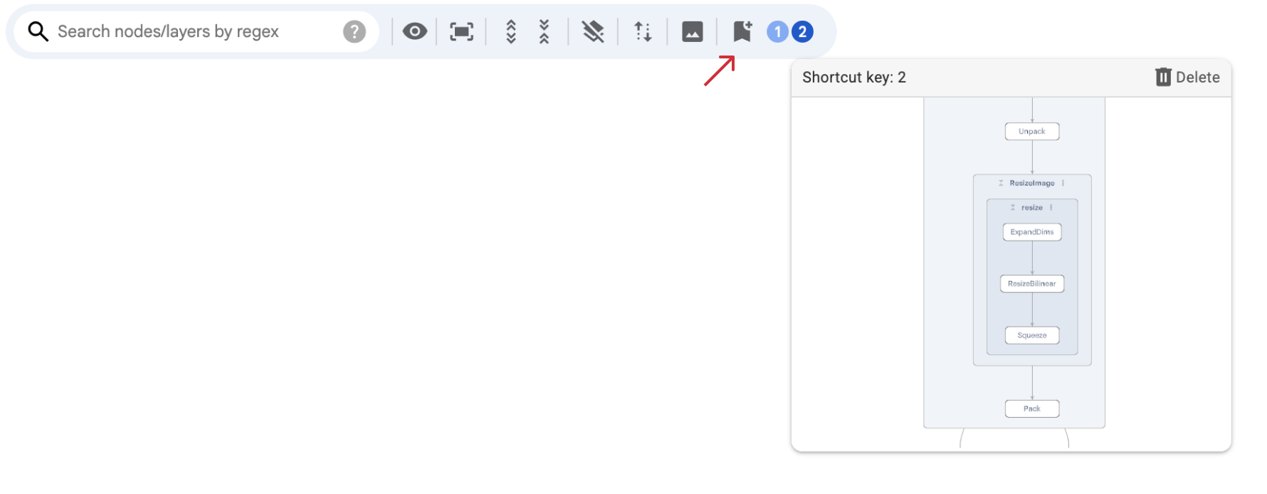
Once you save a state, a numbered button appears on the toolbar. Click this button to restore that view instantly. For even faster access, use number keys (1, 2, 3, etc.) as shortcuts. Hover over a saved state button to preview its screenshot and a button to delete the state. You can save up to 9 states at a time.
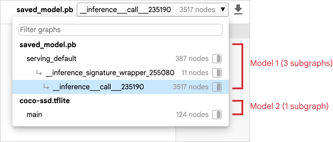
When you've selected multiple models, the visualization page will initially show the largest subgraph from your first model. You can easily switch between models and their subgraphs using the model graph selector in the top-right corner. It shows models and subgraphs in a tree-like view, and supports simple filtering for subgraphs.
Tip
There is a "download" button next to the model graph selector. Clicking it will save the currently visualized graph in a processed JSON format. You can add the downloaded JSON graphs directly in the Model Explorer home page, and they are typically much smaller and process much faster than original model files since they are post-transformed and will bypass the adapter transformation process.
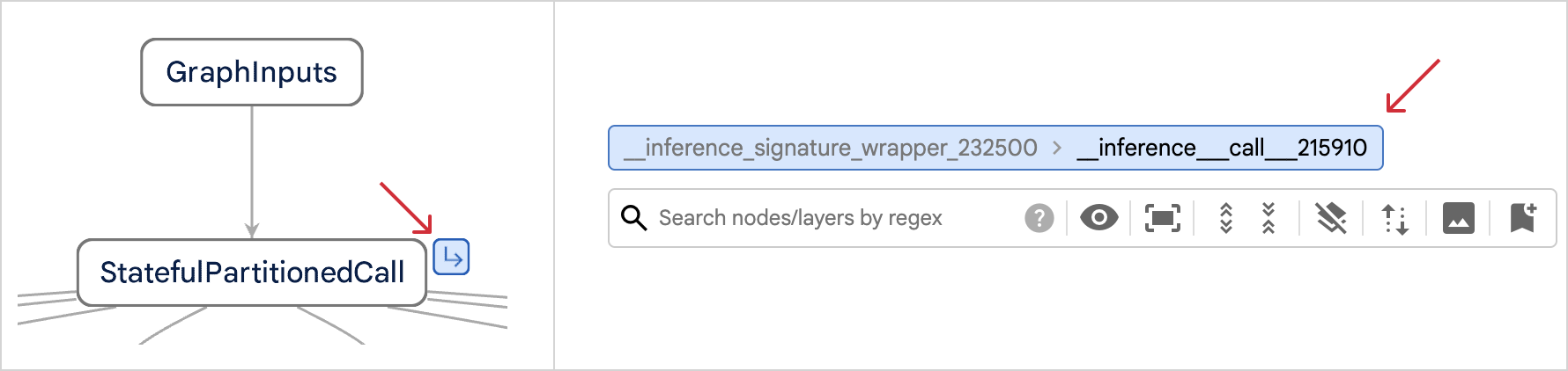
If a model contains multiple connected graphs (e.g., a parent graph with subgraphs), Model Explorer will display a "jump" icon on the node leading to the subgraph. Click the "jump" icon to navigate directly to the associated subgraph. A breadcrumb will appear above the toolbar, allowing you to easily jump back to the previous graph.
Split pane view allows users to view two arbitrary model graphs side-by-side for easy comparison. To view different graphs in a split pane view, make sure to select multiple models from the home page.
To open split pane view, select the split pane icon for your desired graph from the model graph selector.
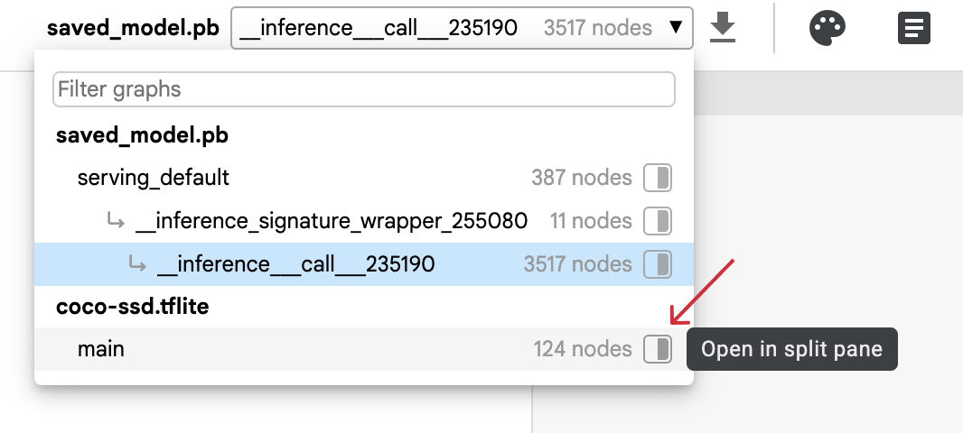
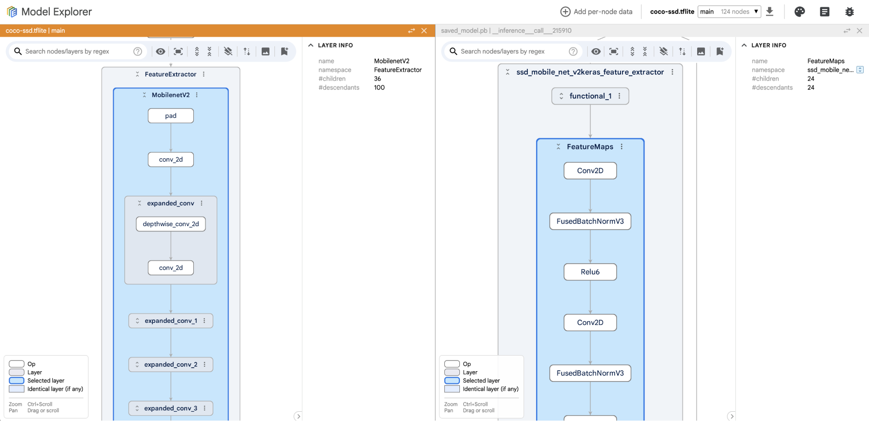
A view of the selected graph will appear on your screen. Both views are fully functional. You can switch and close views using the swap and close buttons located in the top right of each panel. You can also resize views by dragging the resizer in the middle.
To help with debugging model issues, Model Explorer allows you to upload custom node data JSON files. The JSON file provides per-node custom values (e.g. performance latency), as well as color mapping configs so that Model Explorer can automatically color-code nodes based on its custom value. Using custom node data is a powerful way to visualize your own data directly on the model graph, making it easier and more intuitive to find patterns and gain valuable insights into model's behavior.
Note
The custom data is only for op nodes, not layer nodes.
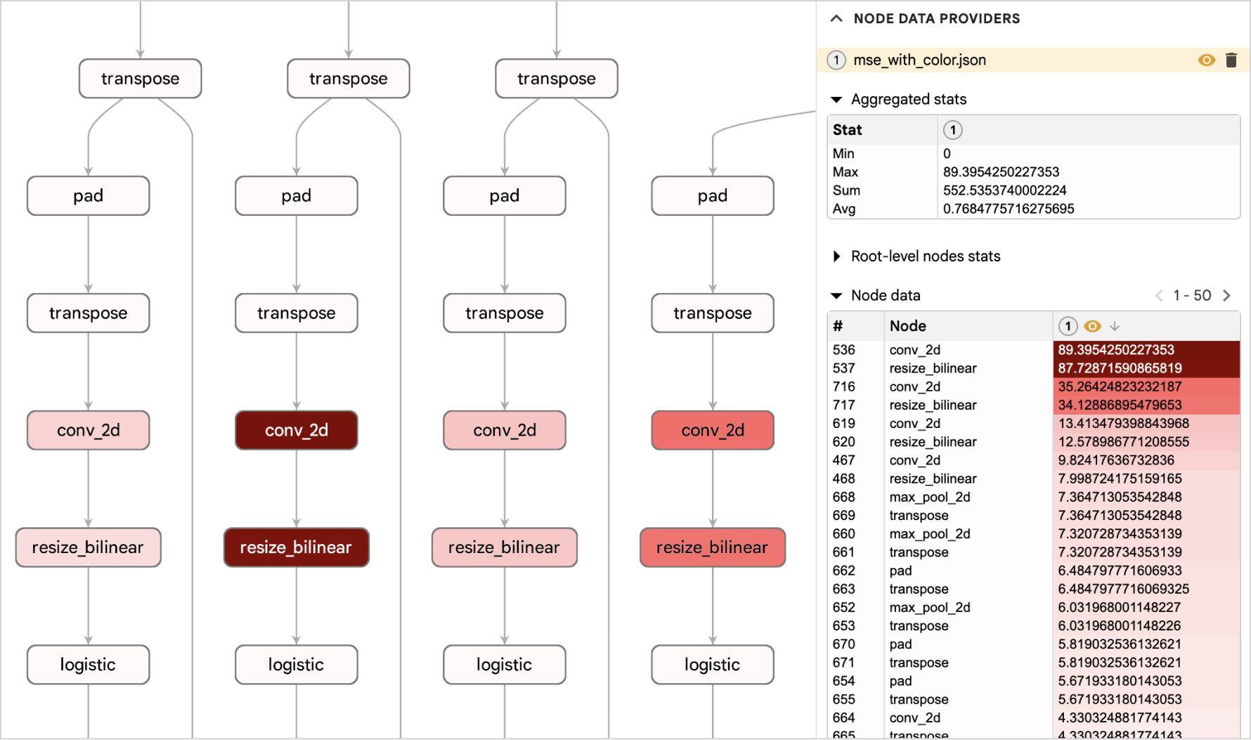
The following screenshot illustrates a real-world debugging scenario using custom node data. We identified model quantization issues by comparing accuracy differences between a float32 model and its quantized int8 model for each node, then visualized these results directly on the graph using custom node data. The visualization result clearly pinpointed problematic Conv2D nodes located towards the end of the model, providing actionable insights for further investigation.
We provide a set of Python APIs to help you create custom node data and serialize it into a JSON file. See the API guide for instructions. You can also create this file easily from other languages/tools by using the following JSON schema. Refer to the comments in node_data_builder.py as the official documentation.
{
  [key: graphId]: {
    results: {
      [key: nodeIdOrAnyOutputTensorName]: {
        value: number;
        bgColor?: string;
        textColor?: string;
      }
    };

    thresholds?: Array<{
      value: number;
      bgColor: string;
      textColor?: string;
    }>;

    gradient?: Array<{
      stop: number;
      bgColor?: string;
      textColor?: string;
    }>;
  }
}To upload the custom node data JSON files to Model Explorer, click the "Add per-node data" button in the app bar at the top, then click the "upload" button to upload the JSON files from your computer.
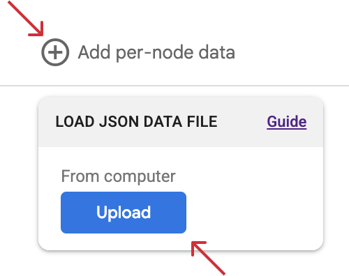
After the files are uploaded and processed, the data will be shown in side panel and in the model graph.
Data in side panel:
A new "Node data provider" section will appear in the side panel. What is shown in this section depends on what is currently selected in the graph.
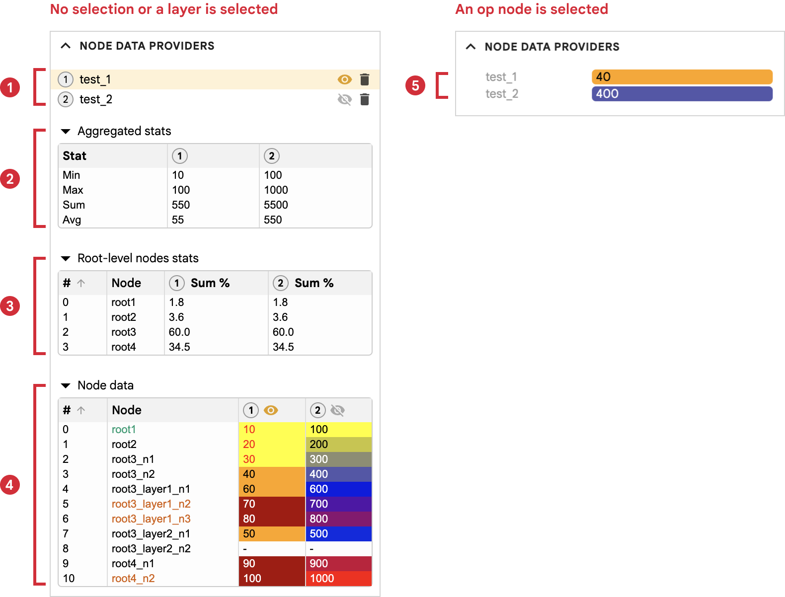
-
Node data index:
A list of all the uploaded node data files. Use the "eye" icon to control which one to be visualized in the model graph. Use the "delete" icon to delete them.
-
Aggregated stats table:
It shows the aggregated stats for all the op nodes under the currently selected layer.
-
Immediate child nodes stats table:
It shows the stats for the immediate child nodes (layers + ops) under the currently selected layer. It supports the following stats:
- Sum%: the percentage of the summed value for each child relative to the total sum of all the op nodes in the selected layer.
-
Color-coded op node values table:
It shows the individual value for each op node under the currently selected layer. The background and the label colors are calculated from the color configs in the JSON file. You can click on a node label to directly jump to that node in the model graph. Click the "eye" icon on the column header to specify which node data file to be visualized on the graph (same functionality as in the node data index)
-
Custom node values for the node:
When an op node is selected, the section will show the color-coded custom node values from all JSON files.
Tip
You can collapse/expand a table by clicking on the triangle icon. All table columns are sortable by clicking on the column header.
Data in model graph:
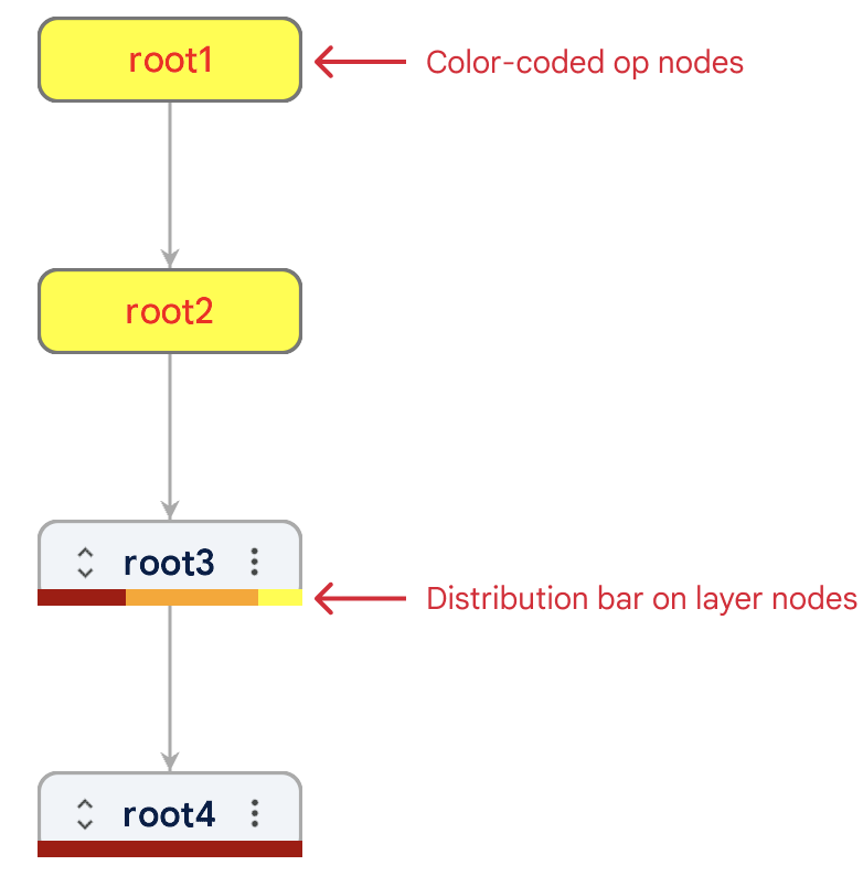
In model graph, op nodes will be rendered with colors calculated from the color mappings and node values in the JSON file, and layer nodes display a color bar representing the distribution of background colors for all op nodes within that layer, providing a quick visual overview of potential hotspots or patterns.
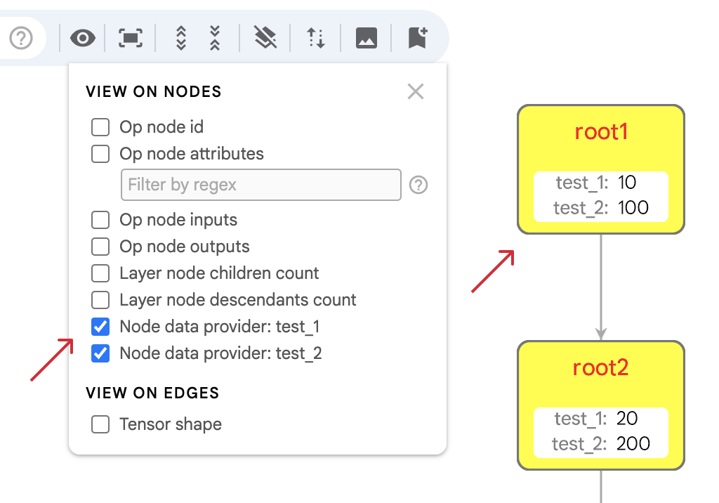
The uploaded custom node data files become available in the "View on node" menu. Selecting them will show the corresponding node data values on nodes directly.
Node styler allows you to create "rules" that use custom queries to match nodes and apply styles to them.
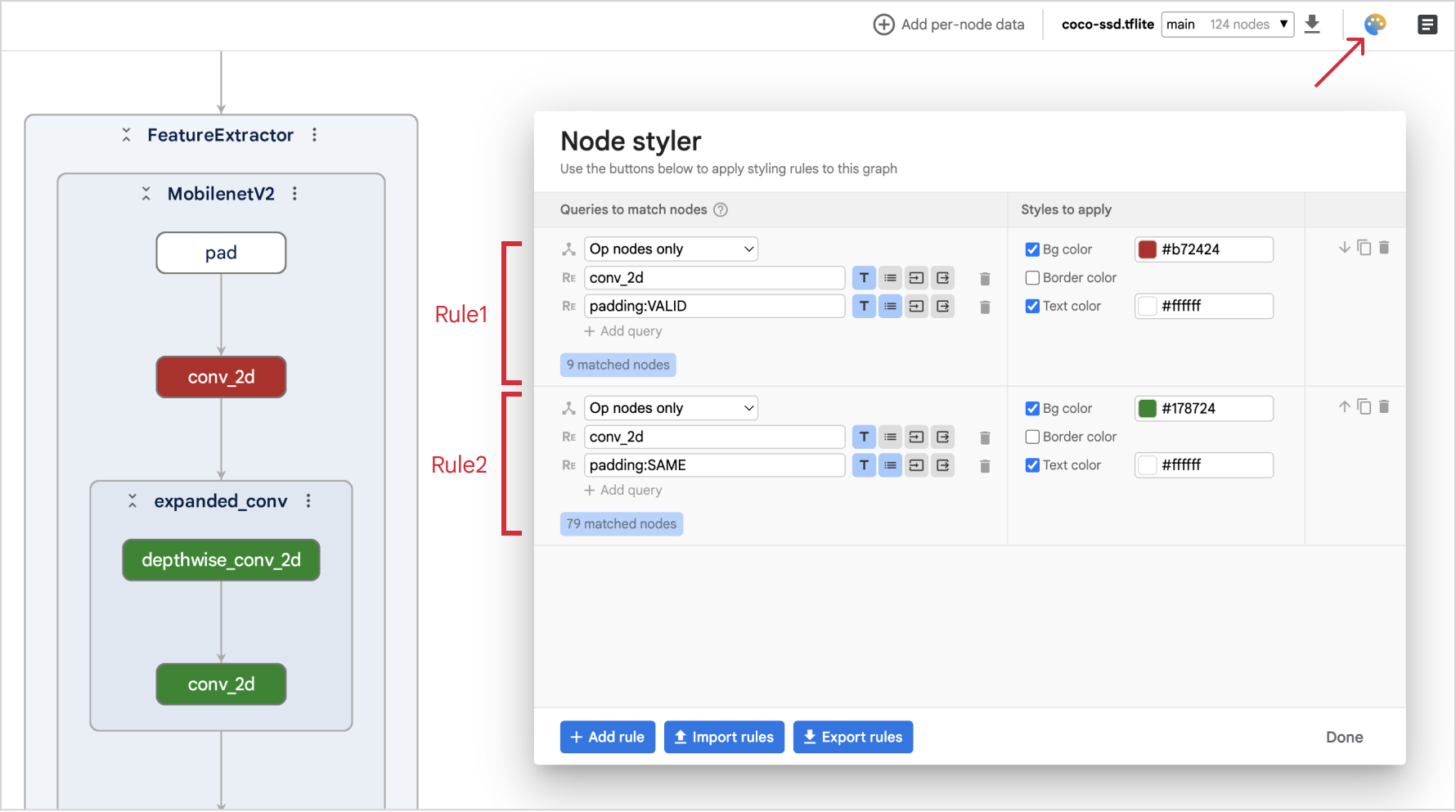
The screenshot above shows two rules we created. The first rule matches nodes with the following queries (they are AND'd together):
- The node should be an op node.
- The node label should match the "conv_2d" regex.
- The node should have an attribute "padding" with "VALID" value.
In the "styles" column, we applied a red background color and a white text label to the matched nodes.
The second rule is almost the same as the first rule, but targets nodes with an attribute "padding:SAME", applying a green background instead of red.
The node styler rules persist in browser's local storage, and can be easily exported (to a JSON file) and imported.
Click the "settings" icon in the home page for a list of advanced settings. For each setting item, hover over the "help" icon to see how it works. All settings are stored in browser's local storage.

Key UI states, such as selected nodes, expanded layers, and split-pane, are encoded directly in the URL. If you accessed your model by providing its full absolute path on the home page, you can bookmark this URL to easily restore both the model graph and the UI states.
Note
The URL won't work if you loaded the model using the "Select from your computer" button. It also won't work when opened on somebody else's machine since Model Explorer server runs locally on your machine by default.