Chenyu You, Qingsong Yang, Hongming Shan, Lars Gjesteby, Guang Li, Shenghong Ju, Zhuiyang Zhang, Zhen Zhao, Yi Zhang, Member, IEEE, Wenxiang Cong, and Ge Wang*, Fellow, IEEE
- Numerous methods have been designed for noise reduction in LDCT. These methods can be categorized as follows:
-
Sinogram filtering-based techniques : these methods directly process projection data in the projection domain, bowtie filtering, and structural adaptive filtering. The main advantage of these methods is computational efficiency. However, they may result in loss of structural information and spatial resolution in LDCT acquisition
-
Iterative reconstruction(IR) : IR techniques may potentially produce high signal-to-noise ratio (SNR). However, these methods require substantial computational resource, optimal parameter settings and accurate modeling of noise properties
-
Image space denoising techniques : these techniques can be performed directly on reconstructed images so that they can be applied across various CT scanners at a very low cost. Examples are non-local means-based filters, dictionary-learning-based K-singular value decomposition (KSVD) method [18] and the block-matching 3D (BM3D) algorithms. Even though these algorithms greatly suppress noise and artifacts, edge blurring or loss of spatial resolution may still remain in the processed LDCT images.
- Deep Learning : Recent studies demonstrate that deep learning (DL) techniques have yielded successful results for noise reduction in LDCT.
-
Chen et al. [31] proposed a pioneering Residual Encoder-Decoder convolutional neural network (REN-CNN) to predict NDCT images from noisy LDCT images. This method greatly reduces the background noise and artifacts. However, the major limitation is that the content of the results is blurry since the method is iteratively minimizing the mean-squared error per voxel between generated LDCT and the corresponding NDCT images.
-
To cope with this limitation, generative adversarial networks (GANs) [36] provide a feasible solution. The generator G learns to capture a real data distribution Pr and the discriminator D attempts to discriminate between the synthetic data distribution and the real data distribution. Note that the loss used in GAN, called adversarial loss, measures the distance between the synthetic data distribution and the real data distribution in order to improve the performance of G and D. Here the GAN uses arXiv:1805.00587v2 [cs.CV] 4 May 2018 2 Jensen-Shannon (JS) divergence to evaluate the similarity of the two data distributions [36]. However, several problems still exist in training GAN, such as unstable training or nonconvergence issues.
-
To cope with these issues, Arjovsky et al. introduced the Wasserstein distance instead of Jensen-Shannon divergence to improve the stability of the neural network training [37]. We discuss more details in Section II-D3.
-
Our previous work [33], which first introduced perceptual loss to capture perceptual differences between denoised LDCT images and the reference NDCT images, provides the perceptually better results for clinical diagnosis but yields low scores in image quality metrics.
-
To better render the underlying structural information between LDCT and NDCT images, we adopt a 3D CNN model as a generator based on WGAN which can integrate spatial information to enhance the image quality and yield 3D volumetric results for better diagnosis.
-
To consider the structural and perceptual difference between generated LDCT images and gold-standard, structure-sensitive loss can enhance the accuracy and robustness of the algorithm. Different from [33], we replace perceptual loss with the combination of L1 loss and structural loss to capture local anatomical structures while reducing background noise.
-
To better compare the performance of the 2D and the 3D models, we perform extensive investigations and evaluations on their convergence rate and denoising performance.

-
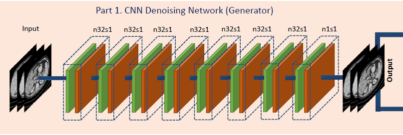
The generator G consists of eight 3D convolutional (Conv) layers. The first 7 layers each have 32 filters and the last layer has only 1 filter.
-
Based on our practical experience, the odd-numbered convolutional layers have 3 * 3 * 1 filters, and the even-numbered convolutional layers have 3 * 3 * 3 filters. The size of the extracted 3D patches used as the input is 80 * 80 * 11.
-
See Fig. 1. Note that the variable n denotes the number of the filters and s denotes the stride size which means the step size of the filer when moving across the image so that n32s1 stands for 32 feature maps with stride one pixel.
-
A pooling layer after each Conv layer may lead to loss of subtle textural and structural information, and spatial inconsistency in training stages. Therefore, the pooling layer is not applied in this network.
-
Next, the Rectified Linear Unit (ReLU) [41] is utilized as the activation function after each Conv layer. The benefits to utilize ReLu are as follows. First, it produces nonlinear interactions with its input, which in turn prevents the generated results from being equal to a linear transformation of the input. Second, it is crucial to maintain the sparsity in the inputs to each Conv layer to perform effective feature extraction in high-dimensional feature space

- The proposed 3D SSL function measures the patch-wise error between the 3D output from 3D ConvNet and the 3D NDCT images in spatial domain. This error was back-propagated [42] through the neural network to update the weights of network.
-
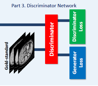
The discriminator D used in this network is made up of six convolutional layers with 64, 64, 128, 128, 256, and 256 filters and the kernel size of 3 * 3. Two fully-connected (FC) layers produce 1024 and 1 feature maps respectively. Each layer is followed by a leaky ReLU in the manner of max(0; x) - a max(0;-x) where a is a small constant.
-
A stride of one pixel is applied for odd-numbered Conv layers and a stride of two pixels for even-numbered Conv layers. The input fed to D has the size of 64 * 64 * 3, and is the output of G. The reason why we use a 2D filter in D is to lower the computational complexity. Since the adversarial loss between each two adjacent layers in one volumetric patch contribute equally to the weighted average in one iteration, it adds no computational expense and also takes into account spatial correlations. Following the suggestion in [37], we removes the sigmoid cross entropy layer in D.
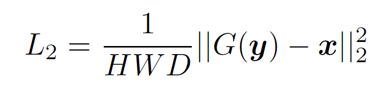
- L2 loss: The L2 loss can efficiently suppress the background noise, but it makes the denoised results unnatural and blurs the image contents. H, W, D stand for the height, width, and depth of the 3D image patches, respectively, x denotes gold-standard images (NDCT), and G(y) represents the generated images from source (LDCT) images y. It is worth noting that since L2 loss has appealing properties of differentiability, convexity, and symmetry, the mean squared error (MSE) or L2 loss is still a popular choice in denoising tasks [45].
- L1 loss: Compared with L2 loss, L1 loss does not over-penalize large differences or tolerate small errors between denoised images and gold-standard images. Thus, L1 loss can alleviate some limitations of L2 loss we mentioned above. Additionally, L1 loss enjoys the same fine characteristics as L2 loss, like a fast convergence speed.

-
Adversarial loss: The improved Wasserstein distance with the regularization term proposed in [43] is expressed as above.
-
where the first two terms are computed for Wasserstein distance and the third term is the gradient penalty term. It is worth noting that z denotes G(y) for brevity.
-
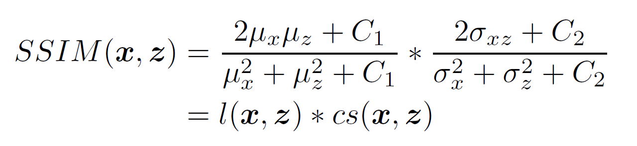
Structural loss: Medical images have strong 3D image correlations; their voxels demonstrate strong interdependencies which carry diagnostic information. Structural similarity index (SSIM) [44] and Multi-scale structural similarity index (MS-SSIM) [46] are better perceptually motivated metrics than mean-based metrics [44] since SSIM and MSSSIM quantify structure errors (difference) between reference images and input images, and take advantage of the characteristics of the human visual system (HVS).
-
where C1,C2 are constants and mx, mz, 0x, 0z, 0xz denote local means, standard deviation and cross-covariance of the image pair (x; z) from G and the corresponding NDCT respectively.

- Multiscale SSIM provides more flexibility for better generalization than the single-scale method, including different resolutions and local distortions

- L1 loss can deliver noise suppression and increase SNR. However, it blurs anatomical structures to some extent. In contrast, structural loss can encourage less smoothness compared with L1 loss and keep high contrast resolution. To capture merits of both loss functions, the structural sensitive loss (SSL) is expressed above. where τ is the scale weight to control the balance between structure preservation in the first term (from Eq. 9) and noise suppression in the second term (from Eq. 4).

- However, these two methods may inevitably lose some important diagnostic features so adversarial loss is incorporated in our work to maintain texture and structure features. In summary, the overall objective function of SMGAN is expressed above.
-
Data Set: real clinical dataset, published by Mayo Clinic for the 2016 NIH-AAPM-Mayo Clinic Low Dose CT Grand Challenge
-
For limited data, in order to improve generalization performance of the network and avoid over-fitting, we adopt the famous ”10-fold cross validation” strategy
-
For data preprocessing, first, we apply the overlapping strategy in cropping over 100,000 pairs of training and label patches and over 5,000 pairs for validation from remaining patient images with the same size of 80 × 80 × 11. Then, the ”10-fold cross validation” strategy is adopted. Next, the CT Hounsfield Unit (HU) scale is normalized to [0, 1] before the images are fed to the network.
-
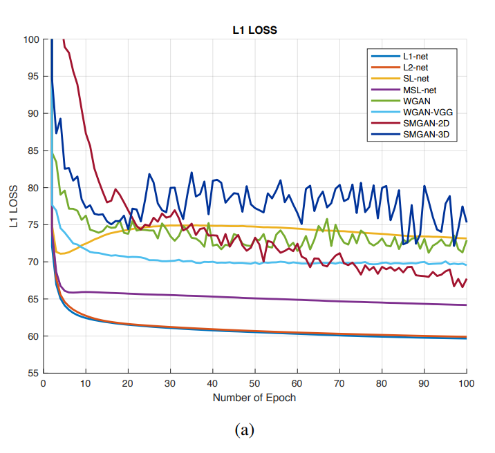
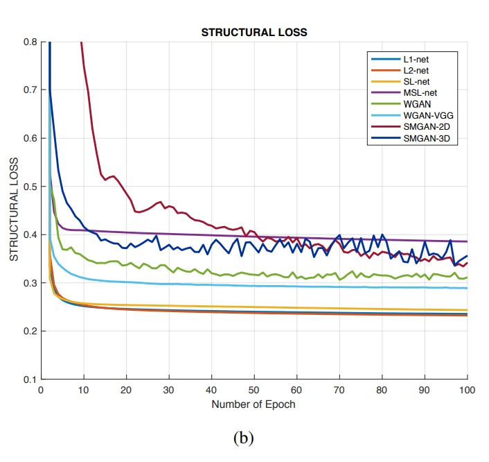
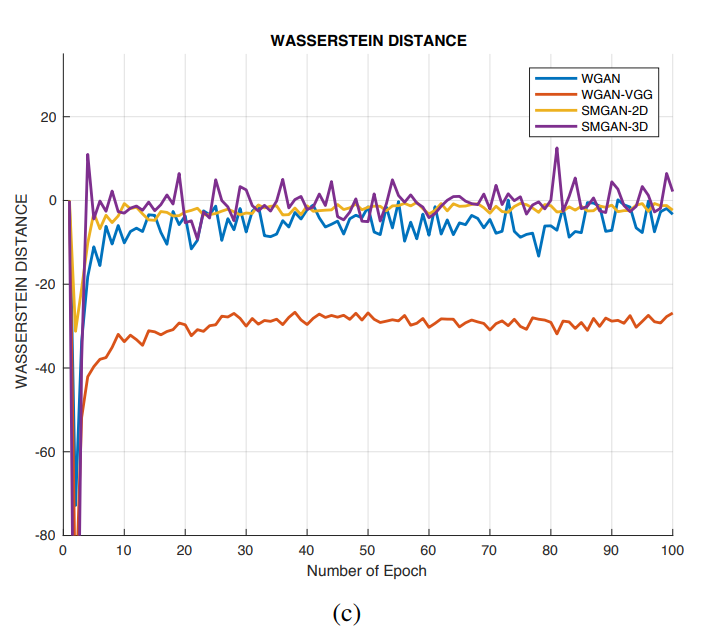
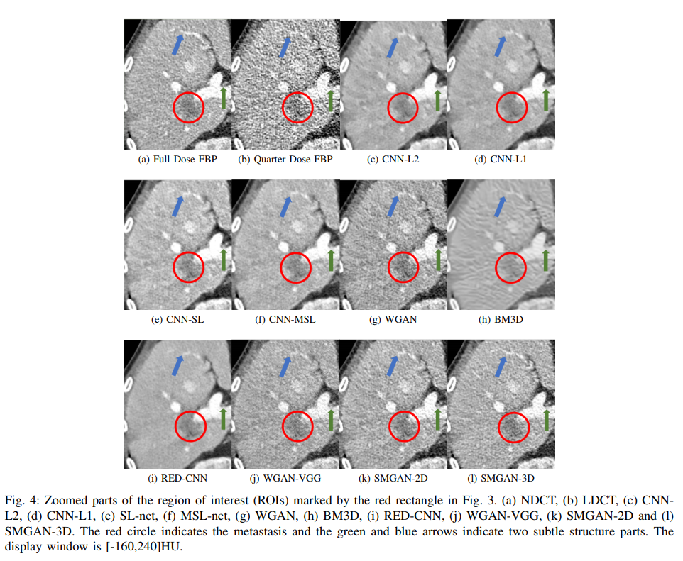
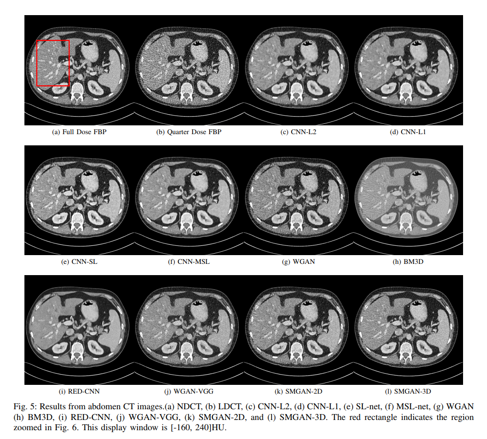
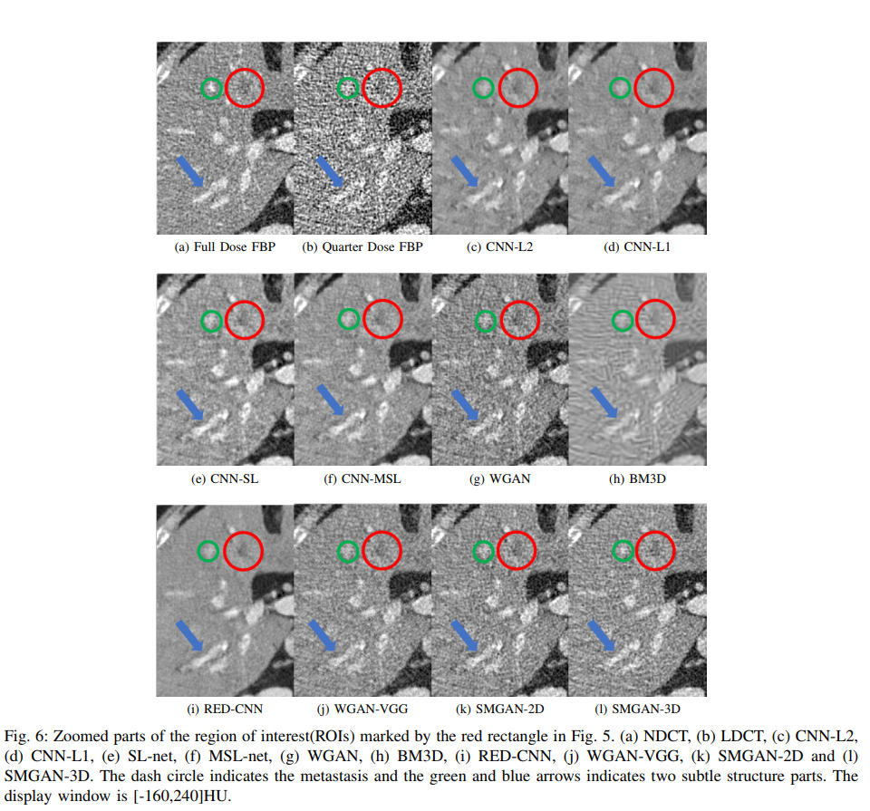
For qualitative comparison, in order to fully validate the performance of our proposed methods (SMGAN-2D and SMGAN-3D), we compare with eight state-of-the-art denoising methods, including CNN-L2 (L2-net), CNN-L1 (L1- net), structural-loss net (SL-net), multi-scale structural-loss net (MSL-net), WGAN, BM3D [23], RED-CNN [31], and WGAN-VGG
- Comparison among loss function value versus the number of epochs with respect to different algorithms
- CT image results

- Visual assessments by three radiologist readers

-
Although our proposed network has achieved high-quality denoised LDCT images, there are still some limitations. First and foremost, the feature edges in the processed results may 13 still have blurring effects.
-
Secondly, some structural variations between NDCT and LDCT did not perfectly match in each pixel. A better way to incorporate a dynamic routing model to enhance information correlation between NDCT and LDCT is to design a novel complex network to improve the transformation modeling capability, which is the work we have started.