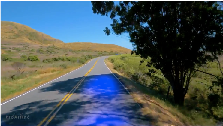
We approach the problem of road detection for autonomous vehicles by using a machine learning approach on images from a dash-mounted camera. Considering the challenge presented by rural and poorly marked roads, we develop and optimize a fully convolutional network (FCN), and demonstrate the model’s robustness on a variety of roads. Finally we discover a limitation in our model, and devise method-ologies for automatically generating additional training data that will counteract this. The result of our method can be seen in the following animation.


Research into autonomous driving is becoming more and more popular. Road detection is an essential ability for safe navigation of a car by either a human driver or a computer. A road detection program also represents an intermediate step to full autonomy, with the ability to alert an inattentive driver when they drift from their lane. Vehicles this this capability are on the road today, and continued research into the problem will continue for some time. Our project is to use a machine learning approach to this problem, trying to help a computer detect the road by using data from front facing camera or dash cam, a cheaper alternative to radar or lidar. In reviewing methodologies that exist, we noticed a focus on highways and urban roads which are clearly marked by lines and other isolation strips. We sought to design a model that was also robust on rural roads, which are more challenging due to more variabilities and more vague markings. Our first data set, and inspiration for the project, came from a capstone project by Michael Virgo [1]. We sought to understand the models he used, then design modified and optimized models that are accurate for rural roads as well, something Virgo did not explore in his paper.
The number of good datasets available for autonomous driving in rural roads is very limited. We used a combination of KITTI dataset for training and validation, and videos of unlaned roads from youtube for testing purposes. The KITTI dataset we used was labelled, but inappropriately compared to what the CNN network was setup to use during training. The KITTI dataset came with 3D velodyne point clouds, 3D GPS/IMU data and 3D object tracklet (cars, trucks pedestrians) labels, whereas we wanted a dataset containing pixels belonging to edges of the road as labels. Hence we had to manually label all the frames in the dataset.
We used an online tool called labelbox.io, which would allow us to select a rectangular area in each image, and once finished, would return a CSV file with the coordinates of the polygon that was drawn in each frame. All the pixels within this polygon boundary would be labelled as edge pixels of the road. Fig. 1 shows a screenshot of this procedure.

In this problem, we are trying to understand an image at pixel level. There are several approaches for these sorts of problems, including Texton Forest and Random Forest based classifiers. Another classic method and the one we started with is Convolutional Neural Network (CNN) models. Fig. 2 gives an example of a CNN model structure. The training data we have is a group of individual frames from a variety of driving videos. We also have labels for each pixel of each frame in this training data. Our ideal output would be a model that labels every pixel of our input image appropriately. However, we ran into problems trying to do this through CNN models. First, we find that most CNN models end with fully connected layers and fully connected layers can only deal with input of a fixed size, because it requires a certain amount of parameters to "fully connect" the input and output. So that means we have to use frames with identical size, while our training data may have a variety of frame sizes from different driving videos. Secondly, CNN models use pooling layers to aggregate the context, but as a direct result the model also lose the ’where’ information for that context. These issues made it impossible to map the output vector directly onto the input image.

After finding some papers and projects on GitHub, we decided to investigate using FCN (fully convolutional networks) models. FCN models also have convolution layers and pooling layers at first, similar to the structure of a CNN. However, instead of using fully connected layers, FCN models will have upsampling layers and decovolution layers, which are essentially reversed pooling layers and reversed convolution layers. The structure of an FCN model is shown in fig. 3.

This results in the output having the same size as the input. We no longer need to worry out the size of input or how to label each pixel in input frame. We follow a Virgo’s project [1] and decide our prototype model will take this structure:

Notice how the second half of the model mirrors the first. To produce a test video output, we separate the individual frames in the test video and put feed these into our trained model. After we get the output, we use it to build a blue channel image at the activated pixels, which represent the road. We then superimpose our blue channel image on top of the original input frame, and then save these output frames to as an reconstructed video.
The prototype model we use is an FCN model discussed in the previous section. The convolution part consists one Batch Normalization layer, two Convolution+ReLU layers, one MaxPooling layer, three Convolution+ReLU+Dropout layers, one MaxPooling layer, then followed by two Convolu-tion+ReLU+Dropout layers and one MaxPooling layer. The deconvolution part is just the reverse order, just changing the MaxPooling to Upsampling, Convolution to Deconvolution. We trained this model for ten epochs, and found it can deal with the urban roads successfully, but when dealing with rural and countryside cases, the performance was fair at best. We observed some noise when road curves as showed in fig. 5 (the noise marked by red circles). Overall we were not satisfied with this result. So we tried to do some refinements on our prototype and produce some models that could meet our requirements.


We considered two general ways to improve the prototype. The first was to focus on tunig the parameters of the model such as padding strategy, strides size, number of epoch, etc. We assumed that the prototype was not accurate due to an insufficient number of training epochs. Additionally, the prototype use "valid" padding, which we suspect resulted in some pixels around the edge being dismissed in training. We decided to train the model with more epochs and use "same" padding to see if the result is better. After 15 epochs of training, the loss drops from 0.0545 at the beginning to 0.0053 in the end. However, when we applied our new model (FCN_1) to videos, we found that even though the blue mark is more stable when road curves, we found it was overfitting to lane markings, making the unmarked road results worse. These results are shown in fig. 6.


The second way we sought to improve our model was changing the model structure. In our prototype, we increase our filters for each set of convolution layers, going from Conv2D(8, (3, 3)), Conv2D(16,(3, 3)), Conv2D(32, (3, 3), and ending with Conv2D(64, (3, 3)). Since our input frame size is 80*160 pixels, we assumed we could continue the trend in this produce better results without losing additional features. So we add two Conv2D(128, (3, 3)) and Conv2DTranspose(128, (3, 3)) (deconvolution) layers into the center of our prototype model. Given the results from FCN_1, we reverted our training epochs back to 10. We saw that the loss drops from 0.0781 at the beginning to 0.0080 in the end. We tested this new model (FCN_2) on our videos and got following result:


Our original data set contained mainly well marked roads, which was a concern. However our FCN model performed very well with only that training data, even on new test videos with more rural road conditions. However, we still noticed that there are moments when our prediction become very noisy, and we may even lose the accurate prediction on certain frames. It quickly became apparent, that sudden changes in the color of the road, most noticeably darkening from shadows, was what was causing this. This is seen in fig. 8.
We concluded that our training data did not contain enough images with shadows on the road, and therefore our model had overfit to uniform, well-lit roads. This discovery is truly what forced us to take the manual labelling approach described in section 2, in order to produce more samples with these conditions. Though this kind of manually labelling approximately 500 frames served our purpose of training the FCN network, it proved to be a very labor intensive and repetitive job, and we still had not produced enough samples for robustness. Hence we decided use a few techniques from computer vision, to design an algorithm to label the frames automatically, so that we could label a sufficient number of frames for our training data [4] [5]. But this task, as we found out, turned out to be challenging. The main problem we had to overcome was the shadows cast by the trees on the road. Since we were dealing with rural roads, clearly there would be a lot of shadows. Our algorithm is summarized in the flowchart in fig. 9 on the following page.
We first make 2 copies of the image and convert one image to YCbCr colorspace, and do a histogram equalization of the luma part of the image. Next, we take the L2 norm of the individual components of the RGB image, and then divide each component of the RGB image with this L2 norm. Then concatenate the 3 normalized components to get a brighter image with reduced shadows. We then use the following model to project the 2D normalized chromaticity image onto a 1D illumination invariant image:

where θ is the projecting direction, and inv is the 1d shadow free invariant image. R, G, and B are the individual color channels of each frame. We then filter out the noise and outliers using a median filter with a kernel size of 15x15 pixels on both the histogram equalized YCbCr image and the 1D illumination invariant image. This is followed by a dilation operation on both images with a ’line’ structuring element of size 11 pixels, followed by an erosion operation using the same structuring element. The combination these two operations is called morphological closing, and is done to detect edges in a smoothed image. We then use a canny edge detector to detect the edges of the road on both the images. The histogram equalized YCbCr processed image is used to get the left edge of the road, while the RGB processed image is used to get the right edge of the road. The two images are then finally added together to get the edges of both edges of the road. The result of the above described algorithm is shown in fig. 10a and 10b.


Even though this algorithm works quite well for smooth shadows, it fails to properly identify the road edges when the shadows have many interwoven bright and dark areas, such as shadows cast by leaves of a tree, shown in fig. 11a and fig. 11b. Our future work will be to design an algorithm which can filter out such ’rough’ shadows as well, so that the road edges can be detected, and a good set of labels can be obtained. To that end, we are investigating Maximum likelihood estimation to derive the time-invariant reflectance image from a sequence of past images, to get a smooth shadow.