Panorama-Image-Stitching

1. Usage

• Data Preparation (Optional)

  • Place your images under $INDIR

  • Run the following command, which will automatically read the focal lengths of images under $INDIR and create focal_length.csv

    cd code
    python3 read_focal_length.py $INDIR
    # E.g., 
    # python3 read_focal_length.py ../data/home

• Running the Code

  • Command

    cd code
    python main.py [--indir $INDIR] [--desc $descriptor_type] [--blend $blending_ratio] [--e2e] [--save] [--cache]
    # E.g.,
    # python3 main.py --indir ../data/parrington --desc mops --cache

  • Command-line Arguments

    --indir: Default to be ../data/home.
    --desc: Default to be sift, choices=['sift', 'mops']
    --blend: Default to be 0.1. Ratio of overlapped region to be blended.
    --e2e: Flag that specifies whether the images are taken end-to-end. If enabled, the first image is concatenated to the end.
    --save: Flag to determine whether to save the stitched image. If enabled, the stitched image will be saved to '../panorama.png'. If not enabled, the panorama will be displayed in a pop-up window.
    --cache: Flag to specify whether to read preprocessed (cylindrical projected) images from cache. If enabled, read images from cahce_dir 'cy_{dataset}'.

---

2. Pipeline

${\color{orange}Step0:}$ Cylidrical projection

• Given the image coordinates $(x,y)$, the corresponding cylindrical coordinates $(x', y')$ mapped on a flat image is: $$(s\theta, sh) \text{, where } \theta = tan^{-1} \frac{x}{f} \text{, } h=\frac{y}{\sqrt{x^2+f^2}} $$

${\color{orange}Step1:}$ Feature detection

• Harris corner detector

  • For each pixel, compute $R = detM-k(traceM)^2$ for the intensity changes. $M$ is as the follows, where $I_x$ and $I_y$ are the derivatives of image with respect to x and y-axis and $G_{\sigma=5}$ is a 3x3 gaussian kernal

$$M=\begin{bmatrix} S_{xx} & S_{xy} \\\\ S_{xy} & S_{yy} \end{bmatrix} = \begin{bmatrix} G_{\sigma}I_xI_x & G_{\sigma}I_xI_y \\\\ G_{\sigma}I_yI_x & G_{\sigma}I_yI_y \end{bmatrix} $$

• Non-maximum suppression is applied to $R$
  • To accelerate the process, we use a boolean mask (R == cv2.dilate(R, np.ones((3, 3)))), where True values represent unchanged pixels after a 3x3 dilation, indicating local maxima (considered keypoint) in the original response.

${\color{orange}Step2:}$ Feature description

• We've implemented the descriptors of MOPs (refer to MSOP in the slide) and SIFT

• MOPs descriptor

  • reference and method
  • Consider a 40x40 square window around the keypoint, scale it to 1/5 size, rotate it to horizontal, and sample a 8x8 patch centered at the keypoint.
    • We achieve this by applying an affine matrix $M=M_{\text{translate(4, 4)}} \ M_{scale} \ M_{rotate} \ M_{\text{translate2origin}}$ and clip the 8x8 patch from the origin.
  • Do intensity normalization to the patch

• SIFT descriptor

  • reference
  • Break the 16x16 subpatch surrounding a keypoint into 4x4 blocks.
  • In each block, gradients are accumulated into a 8-bin histogram based on gradient orientation $\theta$
    • We adjust $\theta$ relative to the orientation of the keypoint.
  • Gradients contribute to bins based on their magnitude weighted by a Gaussian.
  • After normalization the 8x4x4-dim feature vector, clamp gradients > 0.2 to avoid excessive influence of high gradients

${\color{orange}Step3:}$ Feature matching

• Brute-force

  • Calculate the distance matrix to determine pairwise square root distances between keypoints.
  • Additionaly, we apply ratio test to the matches. If $\frac{L_2(\text{best match})}{L_2(\text{second-best match})} < 0.75$, the match is considered good

${\color{orange}Step4:}$ Image Alignment

• RANSAC

  • For each iteration, randomly selected 6 keypoints and compute their mean shift.
  • If the mean shift yields the most number of inliers, update the best shift estimate to be the mean shifts of these inliers.

${\color{orange}Step5:}$ End-to-end Alignment

• We evenly distribute the accumulated drift in the y-direction across all images.

${\color{orange}Step6:}$ Image blending

• linear blending
  • Within the overlapped region of two images, blend the images horizontally by varying $\alpha$ from 1 to 0 $$I_{blended} = \alpha I_{new} + (1-\alpha) I_{prev} $$

3. Experiments and Comparisons

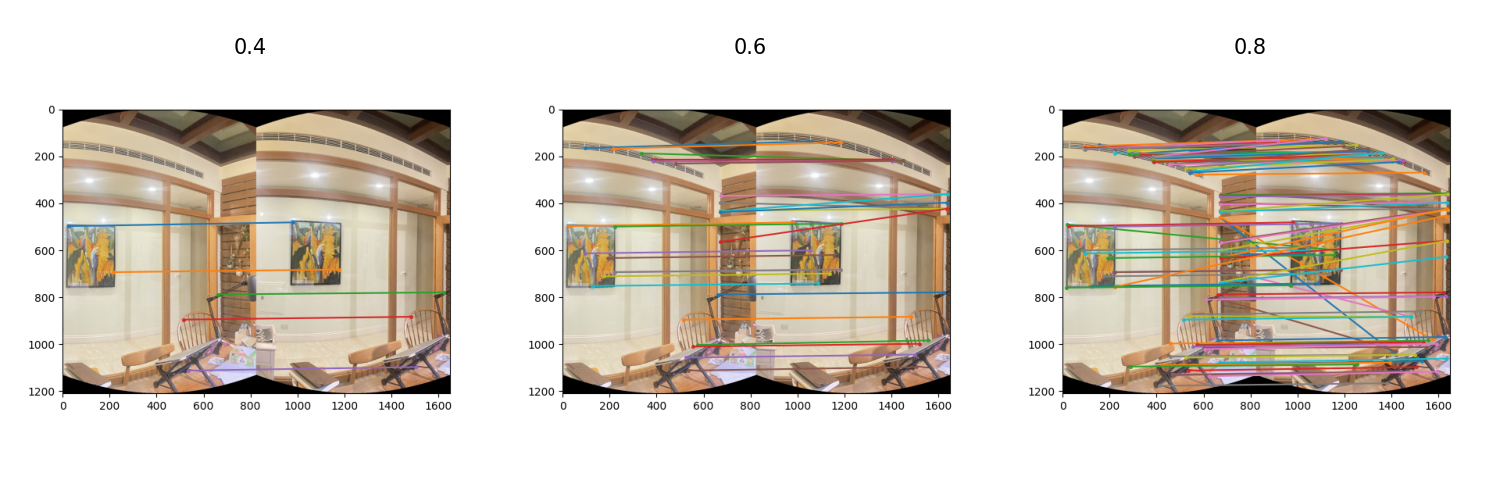
• Feature Matching

  • Ratio Test

    • Specify $t$ such that $\frac{d_1}{d_2} < t$, where $d_1$ and $d_2$ are the nearest and second nearest distance to the query keypoint
    • Lower $t$ gives clearer but fewer matches; higher $t$ gives more but ambiguous matches. Thus, there's a balance between match quality and quantity.
    • We set t=0.8 to maximize the number of points. However, this comes with a trade-off: more iterations of RANSAC during image alignment is required.
    • 

• Image Alignment

  • Let blend ratio = 0 for a clear view, and consider shifts in y

• End-to-end alignment

  • Note that the overflow pixels are appeared at the top/bottom since we use np.roll

• Blending

  • blending ratio

    • Setting blending ratio to 0 means that there is no blending, while setting blending ratio to 1.0 means full blending within the overlapped region.
    • Though higher blending percentages seam the images smoother, there is a trade-off with potential ghosting effects.

4. Result

• Our images

  • 
  • 

• Example images

  • Append the first image to the end
  • 
  •