Vehicle Detection Project

---

Project Writeup / README

Histogram of Oriented Gradients (HOG)

1. HOG features extraction from training images

The HOG features are extracted using the get_hog_features function defined in the project_functions.py file. The function takes an single channel image array and the number of gradient "orientations", the number of pixels per cell in which the histgrams of oriented gradients are computed and the number of cells per block. These paramters are used to tune the hog algorithm.

I started by reading in all the vehicle and non-vehicle images. Here is an example of one of each of the vehicle and non-vehicle classes:

Altough the images are low resolution they still provide a lot of information - in terms of hog algorithm and pixel color information -to be useful for use with the classifier later.

I then explored different HOG parameters (orientations, pixels_per_cell, and cells_per_block). I grabbed random images from each of the two classes and displayed them to get a feel for what the skimage.hog() output looks like.

Here is an example using the R channel of RGB color space and HOG parameters of orientations=8, pixels_per_cell=(8, 8) and cells_per_block=(2, 2):

Below is an image of a car along with the hog algorithm visualization:

2. Final choice of HOG parameters.

I tried various combinations of parameters and the ones that I kept allowed the classfier used later to perform very well on the test dataset. I guess for the kind of images of this application, 8 gradient orientations where enough to capture the signature of the shape of a car and distinguish cars from non cars objects. indeed, using more orientations did not help improve the classifier accuracy.

3. Describe how (and identify where in your code) you trained a classifier using your selected HOG features (and color features if you used them).

I trained a linear SVM using as shown in the classifier.ipynb notebook. I used 0.8 and of the dataset for training the SVM and the remaining data samples to test the accurary which was high at 0.9924.

Sliding Window Search

1. Describe how (and identify where in your code) you implemented a sliding window search. How did you decide what scales to search and how much to overlap windows?

The sliding window search is performed over a region of the image where it is most likely to find cars. That region is scaled down with a 1.5 scale factor. Since I did not vary the window size which is 64 pixels, scaling down at 1.5 seems to be reasonale choice to get a window of size 64 pixels to contain enough information (should it contain a car or part of it) to be classied correctly. The windows also have a 75% overlap. There is a tradeoff between the window size and the overlapping. 64 pixels and 75% overlapping seemed to work well in hindsight as there was very few false positive in classification. below are some windows (image patches extracted with the algorithm)

2. Show some examples of test images to demonstrate how your pipeline is working. What did you do to optimize the performance of your classifier?

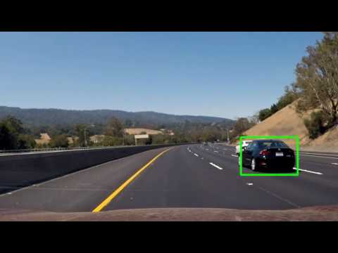
Ultimately I searched on two scales using YCrCb 3-channel HOG features plus spatially binned color and histograms of color in the feature vector, which provided a nice result. Here are some example images:

Video Implementation

1. Provide a link to your final video output. Your pipeline should perform reasonably well on the entire project video (somewhat wobbly or unstable bounding boxes are ok as long as you are identifying the vehicles most of the time with minimal false positives.)

Here's a link to my video result

2. Describe how (and identify where in your code) you implemented some kind of filter for false positives and some method for combining overlapping bounding boxes.

I recorded the positions of positive detections in each frame of the video. From the positive detections I created a heatmap and then thresholded that map to identify vehicle positions. I then used scipy.ndimage.measurements.label() to identify individual blobs in the heatmap. I then assumed each blob corresponded to a vehicle. I constructed bounding boxes to cover the area of each blob detected.

Here's an example result showing the heatmap from a series of frames of video, the result of scipy.ndimage.measurements.label() and the bounding boxes then overlaid on the last frame of video:

Here are six frames and their corresponding heatmaps:

Here is the output of scipy.ndimage.measurements.label() on the integrated heatmap from all six frames:

Here the resulting bounding boxes are drawn onto the last frame in the series:

---

Discussion

1. Briefly discuss any problems / issues you faced in your implementation of this project. Where will your pipeline likely fail? What could you do to make it more robust?

The most tricky part actually was to choose the right heatmap theshold and right buffer size for the number of frame to consider when thresholding the heatmap to find the bounding boxes around cars. To low of a threshold and classification false positives where not eliminated and to high a threshold cars where not tracked correctly. Obviously the higher the threshold the bigger is the number of frames to buffer. The speed of the algorithm is also very unsatifying at about 3 frames per second so as it is, it's not useful for a real application. I would be interesting to replace the SVM algorithm used here with a convolutinal neural network