Introduction to Fly Optic Lobe and Dateset
There are many reasons to choose the fly brain for connectome analyses. First, fruit flies show a relatively complex behavioral repertoire in a relatively small brain, with only ~100,000 neurons. This is particularly important for EM reconstruction because the use of serial electron microscopy is extremely time consuming. This relegates most analyses to small regions (typically under 100 microns x 100 microns x 100 microns).
Second, the fruit fly is a genetic model organism - and hence, any insights resulting from connectomics analyses can be studied by bringing in powerful genetic tools to manipulate elements of the circuits. Indeed, genetic tools exist in the fly for allowing biologists to knock-out or activate specific neurons within a circuit, with high precision. Such tools should prove invaluable in probing the function of neural circuits - and their use should be greatly aided by knowledge of the connections between different neurons in the circuit.
Finally, many fruit fly neurons have characteristic, recognizable arbors. This means that it is possible to use light microscopy to obtain libraries of neuronal shapes (Fly Light Project). Indeed, libraries exist for many of the neurons in the fruit fly's brain. This should aid in connectomics by allowing individual neurons to be recognized, and then compared between different data sets.
Unfortunately, one disadvantage of the fly system is that the structure of the synapses does not reveal their sign. However, the same genetic tools allow parallel efforts to sequence the RNA transcripts within individual cell types. Hence, it should also be possible to obtain the sign of the connections within the circuits.
Within the fly, the optic lobe is an especially appealing neuropil in which to attempt to reconstruct a connectome. Flies are highly visual animals, with the two optic lobes encompassing approximately 50% of the total brain volume.
However, at the same time, the optic lobe is organized retinotopically - with repeating units within each of the different optic lobe neuropils (see below). Therefore, it is not necessary to reconstruct the entire optic lobe, just some representative subregion (covering one or more of the repeating units). Nevertheless, its importance to the animal's survival suggests that a reconstruction of a part of the full lobe would still provide useful information about local computations -
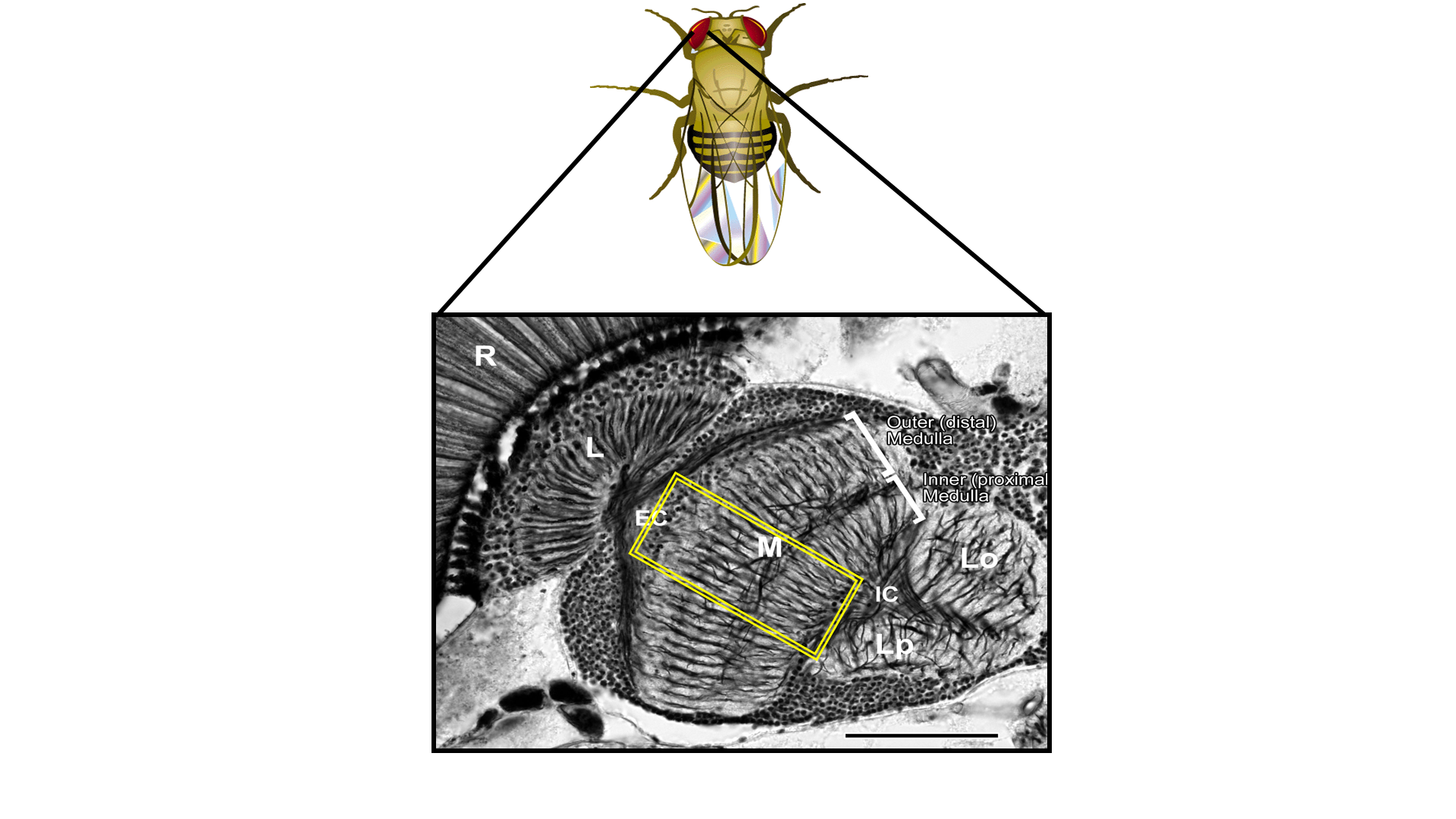
This is a picture of a silver-stained slice through the fly brain showing the basic anatomy of the optic lobes. Just beneath the retina (R), which contains the photoreceptors transducing electrical signals from photons, there are four optic lobes -- lamina (L), medulla (M), lobula (Lo), and lobula plate (Lp).
For orientation, anatomists refer to regions as distal or proximal relative to the center of the brain. The lamina and distal portion of the medulla receive input from the photoreceptors. Conceptually, one can think of the lamina and medulla as conveying parallel units of information to deeper regions of the brain. The lamina is organized into repeating lamina cartridges - each corresponding to a single region of visual space - and, similarly, the medulla is organized into repeating columns.
This repeating structure allows us to have a natural, biological internal test for similarity within repeating circuits (as well as control for external sources of errors). Hence, the statistical analysis of differences between the repeating units of multiple columns would provide a useful way to characterize the variability and error rate of neural circuits (even ones which would, apparently, have to be well conserved).
Finally, in the deeper (proximal) parts of the medulla and lobula, more complex cross-interactions between columns occur (and similarly in the deeper nuclei of the Lobula and Lobula Plate). This allows one to study more complex computations, one example of which being the fly's ability to detection motion: which requires the correlation of two spatially distinct points in visual space.
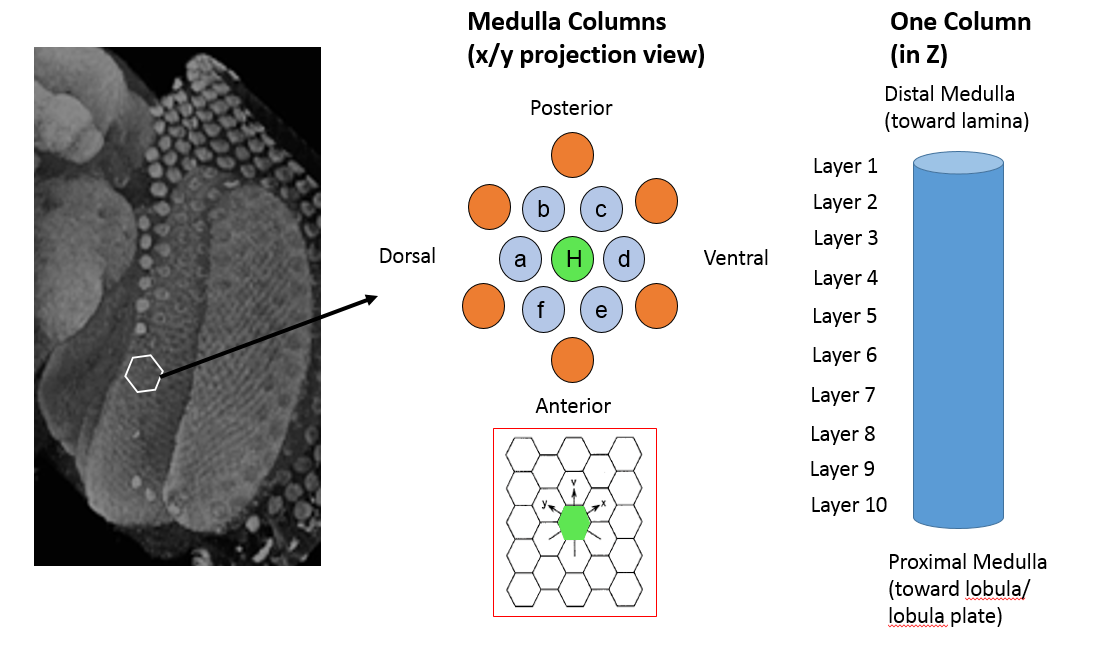
Our most recent (and, as yet, unpublished) reconstruction is focused on seven columns within the medulla, as shown above. The medulla forms hexagonal columnar arrays: one center column with 6 neighbors. Again, one can think of these columns as parallel units in a receptive field. There are two main goals for analyzing 7 adjacent medulla columns:
-
Biologically, adjacent columns when correlated together should uncover the motion detection circuit. Fly EM explored this circuitry in a previous reconstruction that is described in Takemura'13. Our seven column dense reconstruction is larger and more comprehensive than the one in this paper and should offer new insights to this critically important circuit. Furthermore, this circuit is the focus of much research including several theoretical models and general physiological studies. With this rich background, we may be able to produce reasonable hypotheses on the circuit dynamics from structural connectivity, which can then guide further focused experimentation.
-
Presumably, these adjacent columns will be very stereotyped and similar in number of neurons, synapses, etc. It provides an opportunity to study stereotypy, understand biological variability, and examine common motifs over similar columns of neuropil. This may also allow one to distinguish biological sources of variability from the variability due to the reconstruction process.
We define several regions of the seven medulla column (see the image above.)
For purposes of analysis, we label the seven columns with different indicators. The center column (surrounded by 6 adjacent columns) is called the home column (H) and is probably the most thoroughly reconstructed. The other columns are labeled A-F.
Neurons within the optic lobe have characteristic arborizations and, hence, are identifiable as specific cell types. Many prominent medulla neurons are columnar which means they primarily run along the Z-axis of the medulla (also called the proximal/distal axis). There are also tangential neurons that connect the columns. These tangentials run perpendicular to the columnar axis. Seven columns will contain many partial tangential neurons. Further, some columnar neurons actually reside in between columns. For both of these reasons, H is typically considered more completely reconstructed than columns A-F. However, whenever possible, the reconstruction was extended beyond the central seven columns to better capture neurons with arbors within the seven columns that spread out into outer rings.
A single column may contain a single copy or multiple copies of a cell type. For instance, each medulla column has one Mi1 cell type, but there appears to be more than 1 Tm3 neurons per column where they are located at some of the vertices of the hexagonal array. In addition to the columnar structure, the medulla can also be divided into layers in the Z direction. Historically, the medulla has been divided into 10 layers (for more details see Fischbach & Dittrich 1989). Each layer is often defined by specific neurons that arborize in them.
In general, each cell type within the reconstruction can be characterized by the volumes of their arborizations, and their synaptic distributions, within the different columns and layers.
Our EM dataset includes seven complete columns (roughly at the center of the EM images) along with several other columns or partial columns (at the edge of the images). Each voxel is 10nm x 10nm x 10nm. We reconstructed seven medulla columns using techniques found in Plaza et al '14 and Plaza '14. Because the exact boundaries of seven columns are fuzzy and because we did some more tracing outside of the region, the total reconstruction is bigger than the seven columns. Fly EM produced the following which will be available for the hackathon (some data is available publicly on github and is indicated as public):
- Grayscale (8-bit) dataset that is a superset of the segmented data and the seven column reconstruction
- Automatic segmentation for most of the grayscale dataset (64-bit labels where each label is a body ID) -- (the terms body and neuron will mostly be used interchangeably, though a body tends to include neuronal fragments that have not been identified)
- Proofread and refined segmentation for approximately seven medulla columns
- Manually drawn regions of interest to define different compartments of the neuropil (such as the different columns and the different layers in the medulla)
- Synapse locations and pre-synaptic / post-synaptic label assignments (public)
- Cell names and type classification for important bodies, i.e. identifiable neurons (public)
- Skeletons for large neuronal shapes in the dataset (public)
- Contact area between all bodies in the dataset as a label graph. This label graph is also available for each specific ROI.