Fractional-wave-equation: Python module for the numerical solution of nonlinear fractional wave equations
This repository contains python code to numerically calculate the solution U(x,t) of a nonlinear fractional wave equation

on a domain (x,t) ∈ [0,L] × [0,T], and with boundary conditions

where U0(t) and UL(t) are given functions that model time-dependent boundaries.
The exponent α ∈ (1,2) defines the fractional derivative in Eq. (1), and the function D, which depends on ∂xU pointwise, constitutes the nonlinearity.
This python code was written by Julian Kappler to carry out the numerical simulations for the publication Ref. [1]. The numerical algorithm is given in detail in the supplemental section S VII of Ref. [1], and the present code and example notebooks follow the notation of the reference. For the temporal discretization of the fractional derivative, the code uses the method from Ref. [2].
To install the module fractional_wave_equation, clone the repository and run the installation script:
>> git clone https://github.com/juliankappler/fractional-wave-equation.git
>> cd fractional-wave-equation
>> python setup.py installTo run a simulation, the domain (x,t) ∈ [0,L] × [0,T], the functions D, U0, UL, and the order α ∈ (1,2) of the fractional derivative need to specified. For the numerical algorithm, furthermore the spatial and temporal discretization need to be specified.
Here is a simple example (a jupyter notebook with this example can be found here):
import fractional_wave_equation as fwe
L = 10 # spatial domain
Nx = 299 # number of gridpoints inside the spatial domain
T = 10. # temporal domain
Nt = 1000 # number of timesteps
alpha = 1.5 # order of the fractional derivative
# create dictionary for passing to the python module
parameters = {'L':L,
'Nx':Nx,
'T':T,
'Nt':Nt,
'alpha':alpha}
# Define nonlinearity and boundary functions
D = lambda dU_dx: 1 + 2*dU_dx**2 # nonlinearity
U0 = lambda t: 1.*np.exp(-2*(t-2)**2) # boundary at x = 0
UL = lambda t: 0. # boundary at x = L
# instantiate class for nonlinear simulation
nonlinear_equation = fwe.numerical.nonlinear(parameters)
# run simulation
results = nonlinear_equation.simulate(D=D,U0=U0,UL=UL)
# the simulation returns a dictionary, which contains 1D numpy arrays with the
# temporal and spatial grid, as well as a 2D numpy array with the solution U(x,t)
x, t, y = results['x'], results['t'], results['y']
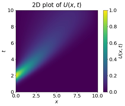
# y[i,j] = U(x[j],t[i])Here is a 2D plot of the solution U(x,t) generated by the above code (as given in this jupyter notebook):
[1] Nonlinear fractional waves at elastic interfaces. Julian Kappler, Shamit Shrivastava, Matthias F. Schneider, and Roland R. Netz. Phys. Rev. Fluids 2, 114804 (2017). DOI: 10.1103/PhysRevFluids.2.114804 / arXiv:1702.08864.
[2] Numerical approximation of nonlinear fractional differential equations with subdiffusion and superdiffusion. Changpin Li, Zhengang Zhao, YangQuan Chen. Chen, Comput. Math. Appl. 62, 855 (2011). DOI: 10.1016/j.camwa.2011.02.045.