document
很久之前写过使用 Mfuzz 和 hclust 的方法来对基因进行聚类和可视化。但是许多人觉得 Mfuzz 出图不是特别美观,此外提供的调整参数也很少,相关推文见:
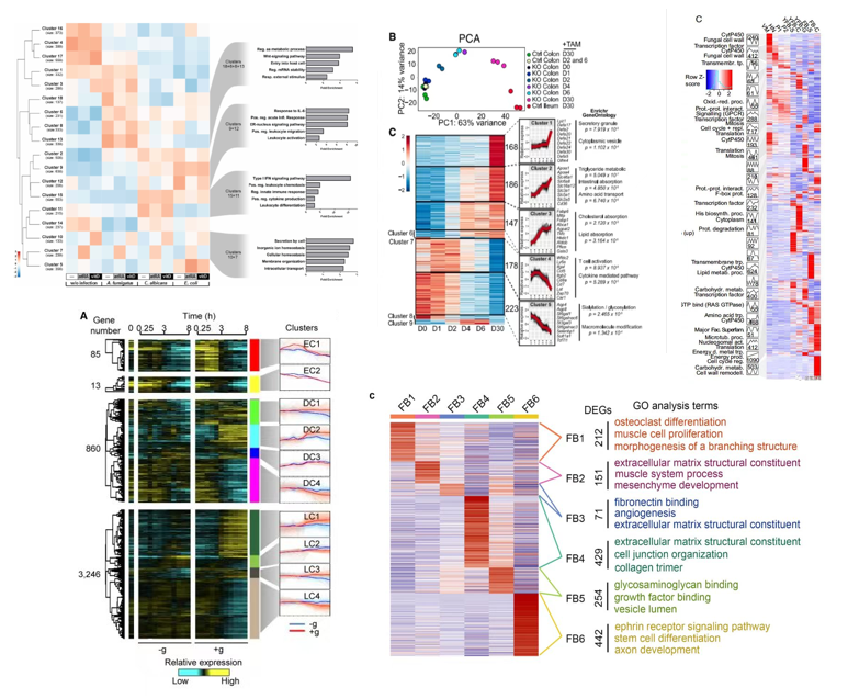
此外我们还会见到 RNA-SEQ 时序分析的 热图 和 表达趋势折线图 及每个亚群的 通路富集结果 可视化在一起,例如:
于是整理整理代码,基于 Mfuzz 的 fuzzy c-means 聚类算法和 ComplexHeatmap 的 row_km 的 Kmeans 聚类对数据进行聚类和可视化,于是产生了 ClusterGVis。这将大大节省科研工作者们写代码和用 Ai 调整美化图片的时间。直接生成发表级图形。
最后致敬感谢这两个包作者的贡献!
github 地址:
觉得有所帮助可以在 github 上留下你的小心心哦!
# install.packages("devtools")
devtools::install_github("junjunlab/ClusterGVis")输入数据是标准化的 tpm/fpkm/rpkm 表达矩阵,有两种方法进行聚类,分别是 Mfuzz 的fuzzy c-means 聚类算法和 ComplexHeatmap 的 row_km 的 Kmeans 聚类算法,用户可根据自己喜好选择。
注意:
聚类是一个随机的过程, 为了保证结果可重复性, clusterData 函数内部设置了随机种子,你可以更改随机种子来改变聚类结果。
...
seed
set a seed for cluster analysis in mfuzz or Heatmap function, default 123.
getClusters 函数计算均方和, 用户可根据拐点确定最佳聚类个数, 首先加载测试数据:
library(ClusterGVis)

# load data
data(exps)

# check
head(exps,3)
#           zygote  t2.cell  t4.cell  t8.cell   tmorula blastocyst
# Oog4   1.3132282 1.237078 1.325978 1.262073 0.6549312  0.2067114
# Psmd9  1.0917337 1.315989 1.174417 1.064756 0.8685598  0.4845448
# Sephs2 0.9859232 1.201026 1.123076 1.084673 0.8878931  0.7174088
绘图:
# check optimal cluster numbers
getClusters(exp = exps)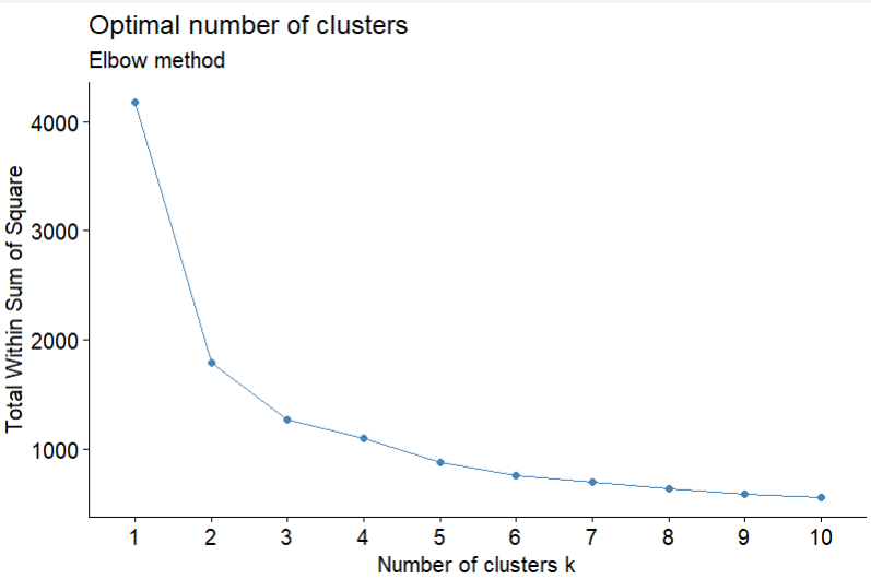
具体聚类的多少你也可以结合热图结果进行选择最佳的数量。
Mfuzz 聚类,选择 8 个聚类数量:
# using mfuzz for clustering
# mfuzz
cm <- clusterData(exp = exps,
                  cluster.method = "mfuzz",
                  cluster.num = 8)
Kmeans 聚类:
# using complexheatmap row_km for clustering
# kmeans
ck <- clusterData(exp = exps,
                  cluster.method = "kmeans",
                  cluster.num = 8)
聚类返回的结果是一个 list,包含了聚类结果的 长数据格式 和 宽数据格式, 当然你也可以使用该数据自己进行绘图。对于 Mfuzz 聚类的结果则会多一列 membership 的信息。
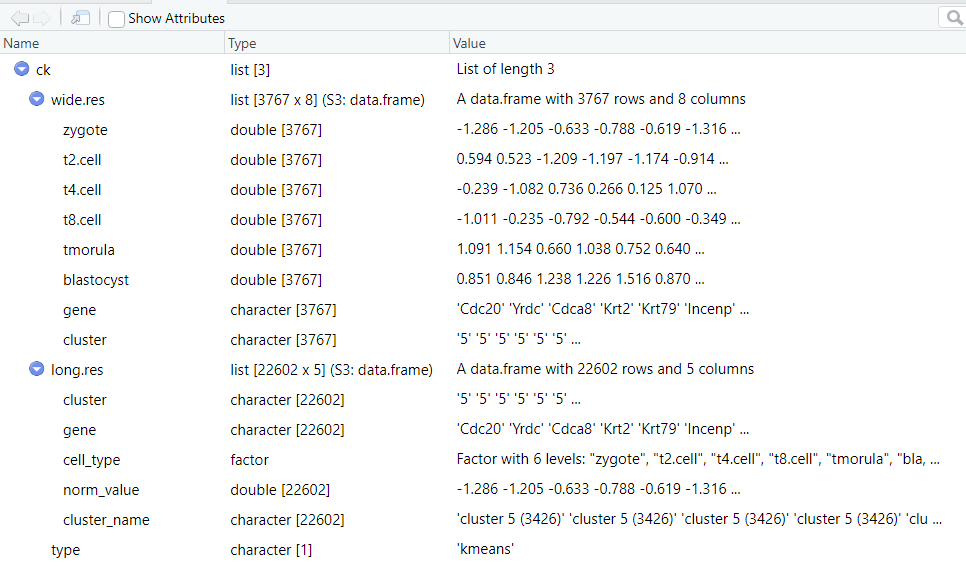
str(ck)
List of 3
 $ wide.res:'data.frame':	3767 obs. of  8 variables:
  ..$ zygote    : num [1:3767] -1.286 -1.205 -0.633 -0.788 -0.619 ...
  ..$ t2.cell   : num [1:3767] 0.594 0.523 -1.209 -1.197 -1.174 ...
  ..$ t4.cell   : num [1:3767] -0.239 -1.082 0.736 0.266 0.125 ...
  ..$ t8.cell   : num [1:3767] -1.011 -0.235 -0.792 -0.544 -0.6 ...
  ..$ tmorula   : num [1:3767] 1.091 1.154 0.66 1.038 0.752 ...
  ..$ blastocyst: num [1:3767] 0.851 0.846 1.238 1.226 1.516 ...
  ..$ gene      : chr [1:3767] "Cdc20" "Yrdc" "Cdca8" "Krt2" ...
  ..$ cluster   : chr [1:3767] "5" "5" "5" "5" ...
 $ long.res:'data.frame':	22602 obs. of  5 variables:
  ..$ cluster     : chr [1:22602] "5" "5" "5" "5" ...
  ..$ gene        : chr [1:22602] "Cdc20" "Yrdc" "Cdca8" "Krt2" ...
  ..$ cell_type   : Factor w/ 6 levels "zygote","t2.cell",..: 1 1 1 1 1 1 1 1 1 1 ...
  ..$ norm_value  : num [1:22602] -1.286 -1.205 -0.633 -0.788 -0.619 ...
  ..$ cluster_name: chr [1:22602] "cluster 5 (3426)" "cluster 5 (3426)" "cluster 5 (3426)" "cluster 5 (3426)" ...
$ type : chr "kmeans"str(cm)
List of 3
$ wide.res:'data.frame': 3767 obs. of 9 variables:
..$ gene : chr [1:3767] "-" "1110007A13Rik" "1110054O05Rik" "1500001M20Rik" ...
..$ zygote : num [1:3767] -0.777 -0.711 -0.75 -0.581 -1.084 ...
..$ t2.cell : num [1:3767] -0.656 -0.319 -0.679 -0.655 -0.716 ...
..$ t4.cell : num [1:3767] -0.39 -0.446 -0.478 -0.502 -0.463 ...
..$ t8.cell : num [1:3767] -0.3616 -0.6177 -0.2645 -0.2745 0.0123 ...
..$ tmorula : num [1:3767] 0.2874 0.1466 0.2731 0.0359 0.5938 ...
..$ blastocyst: num [1:3767] 1.9 1.95 1.9 1.98 1.66 ...
..$ cluster : num [1:3767] 1 1 1 1 1 1 1 1 1 1 ...
..$ membership: num [1:3767] 0.974 0.565 0.992 0.842 0.495 ...
$ long.res:'data.frame': 22602 obs. of 6 variables:
..$ cluster : num [1:22602] 1 1 1 1 1 1 1 1 1 1 ...
..$ gene : chr [1:22602] "-" "1110007A13Rik" "1110054O05Rik" "1500001M20Rik" ...
..$ membership : num [1:22602] 0.974 0.565 0.992 0.842 0.495 ...
..$ cell_type : Factor w/ 6 levels "zygote","t2.cell",..: 1 1 1 1 1 1 1 1 1 1 ...
..$ norm_value : num [1:22602] -0.777 -0.711 -0.75 -0.581 -1.084 ...
..$ cluster_name: chr [1:22602] "cluster 1 (5754)" "cluster 1 (5754)" "cluster 1 (5754)" "cluster 1 (5754)" ...
$ type : chr "mfuzz"visCluster 函数接收来自 clusterData 的结果,支持生成三种绘图结果,包括 折线图,热图,热图+折线(GO 通路) 。
绘制折线图:
# plot line only
visCluster(object = cm,
           plot.type = "line")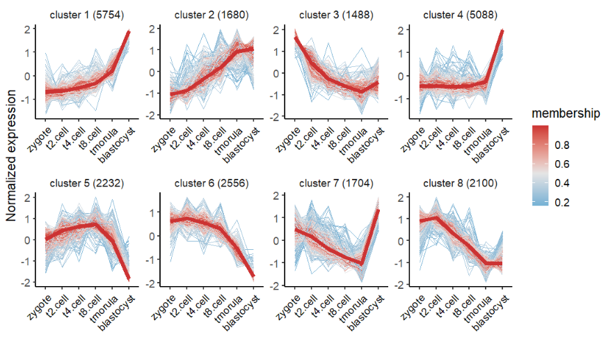
修改颜色:
# change color
visCluster(object = cm,
           plot.type = "line",
           ms.col = c("green","orange","red"))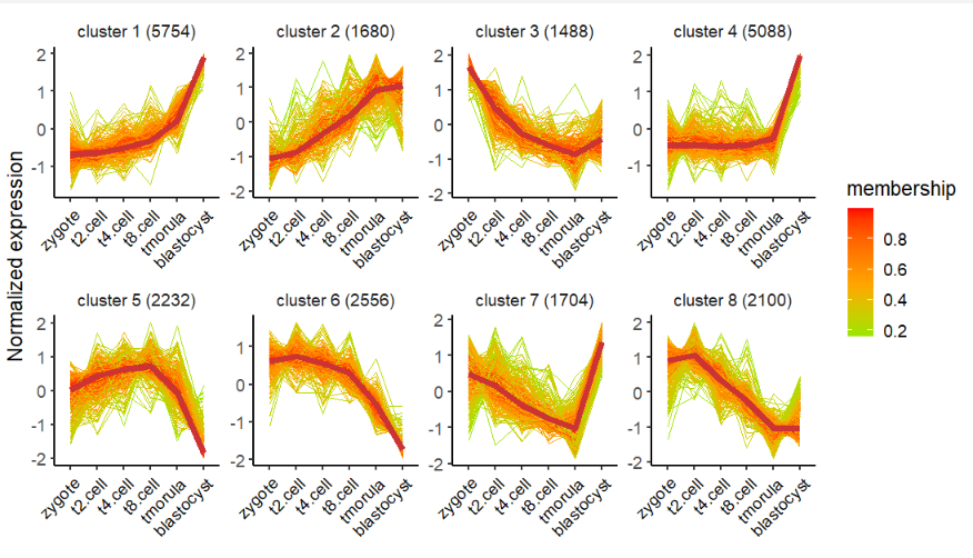
去除中位线:
# remove meadian line
visCluster(object = cm,
           plot.type = "line",
           ms.col = c("green","orange","red"),
           add.mline = FALSE)
kmeans 结果的折线图,因为没有 membership 的信息,所以没有颜色映射:
# plot line only with kmeans method
visCluster(object = ck,
           plot.type = "line")
折线图本质上是 ggplot2 对象,你可以添加其它相关的参数来进行修改细节。
绘制热图:
# plot heatmap only
visCluster(object = ck,
           plot.type = "heatmap")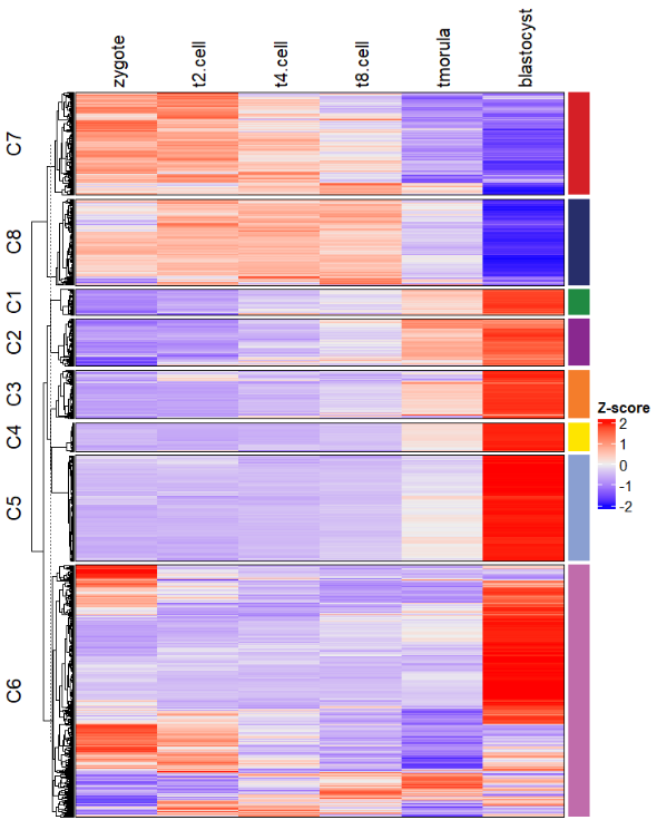
添加其它 Heatmap 相关的参数:
# supply other aruguments passed by Heatmap function
visCluster(object = ck,
           plot.type = "heatmap",
           column_names_rot = 45)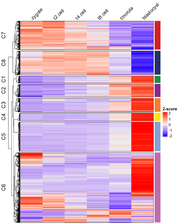
修改注释条颜色:
# change anno bar color
visCluster(object = ck,
           plot.type = "heatmap",
           column_names_rot = 45,
           ctAnno.col = ggsci::pal_npg()(8))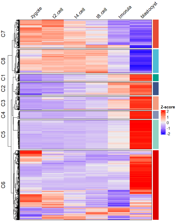
热图加折线图组合,注意窗口显示的图形注释图形并不能很好的对齐,所以将其保存成 pdf 即可:
# add line annotation
pdf('testHT.pdf',height = 10,width = 6)
visCluster(object = ck,
           plot.type = "both",
           column_names_rot = 45)
dev.off()
当然你还可以添加箱线图:
# add boxplot
pdf('testbx.pdf',height = 10,width = 6)
visCluster(object = ck,
           plot.type = "both",
           column_names_rot = 45,
           add.box = T)
dev.off()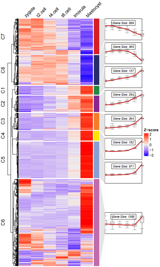
移除折线,修改箱线图颜色:
# remove line and change box fill color
pdf('testbxcol.pdf',height = 10,width = 6)
visCluster(object = ck,
           plot.type = "both",
           column_names_rot = 45,
           add.box = T,
           add.line = F,
           boxcol = ggsci::pal_npg()(8))
dev.off()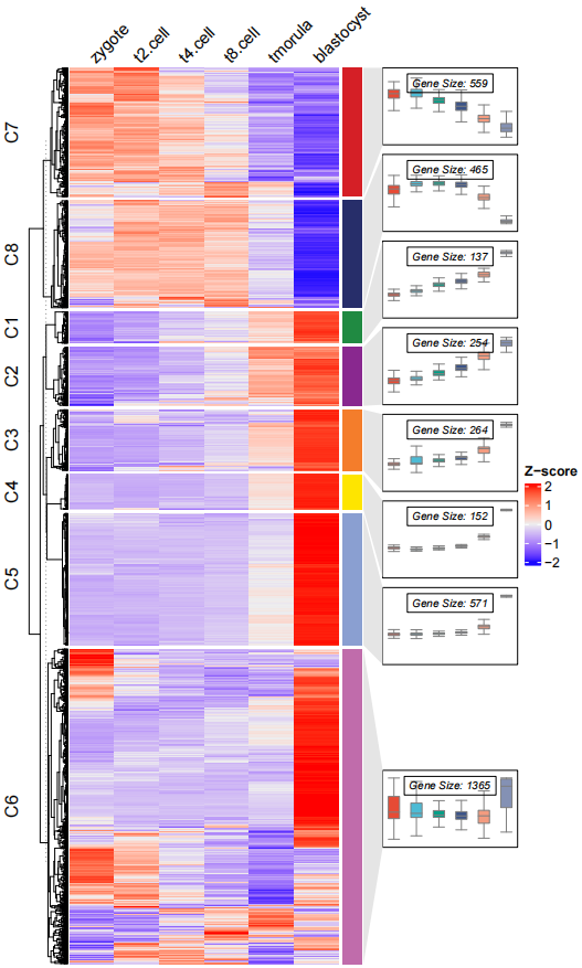
添加 点:
# add point
pdf('testbxcolP.pdf',height = 10,width = 6)
visCluster(object = ck,
           plot.type = "both",
           column_names_rot = 45,
           add.box = T,
           add.line = F,
           boxcol = ggsci::pal_npg()(8),
           add.point = T)
dev.off()
最后你还可以添加富集通路的注释:
# load term info
data("termanno")

# check
head(termanno,4)
#   id                               term
# 1 C1              developmental process
# 2 C1   anatomical structure development
# 3 C1 multicellular organism development
# 4 C2                 system development

# anno with GO terms
pdf('testHTterm.pdf',height = 10,width = 10)
visCluster(object = ck,
           plot.type = "both",
           column_names_rot = 45,
           annoTerm.data = termanno)
dev.off()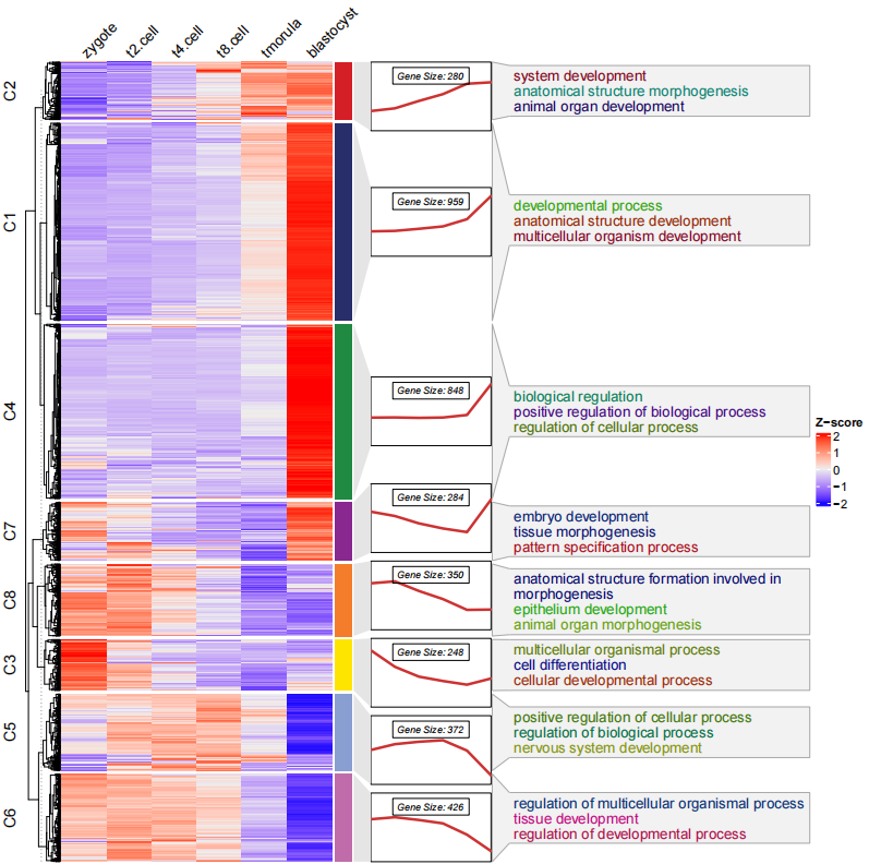
注意富集通路的数据必须是亚群 id 和通路名称, 顺序不能反, 此外 亚群 id 和聚类结果名称(C1...) 保持一致。
你可以看到 通路富集的注释连接与折线图的右边似乎并不太恰当, 因为它是与热图右边的注释条相匹配的,此时你可以调整折线注释的位置
line.side = "left":
# change the line annotation side
pdf('testHTtermCmls.pdf',height = 10,width = 10)
visCluster(object = cm,
           plot.type = "both",
           column_names_rot = 45,
           annoTerm.data = termanno,
           line.side = "left")
dev.off()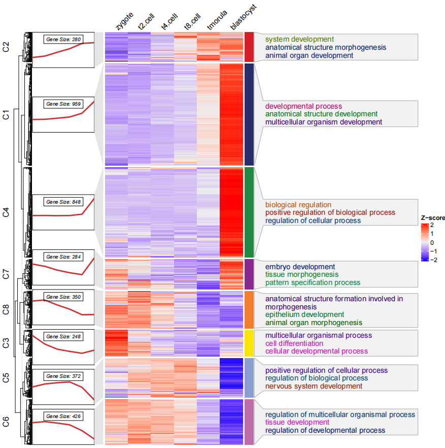
当然你也可以去除左边的聚类树使其更简洁一些:
# remove tree
pdf('testHTtermCmlsrt.pdf',height = 10,width = 10)
visCluster(object = cm,
           plot.type = "both",
           column_names_rot = 45,
           annoTerm.data = termanno,
           line.side = "left",
           show_row_dend = F)
dev.off()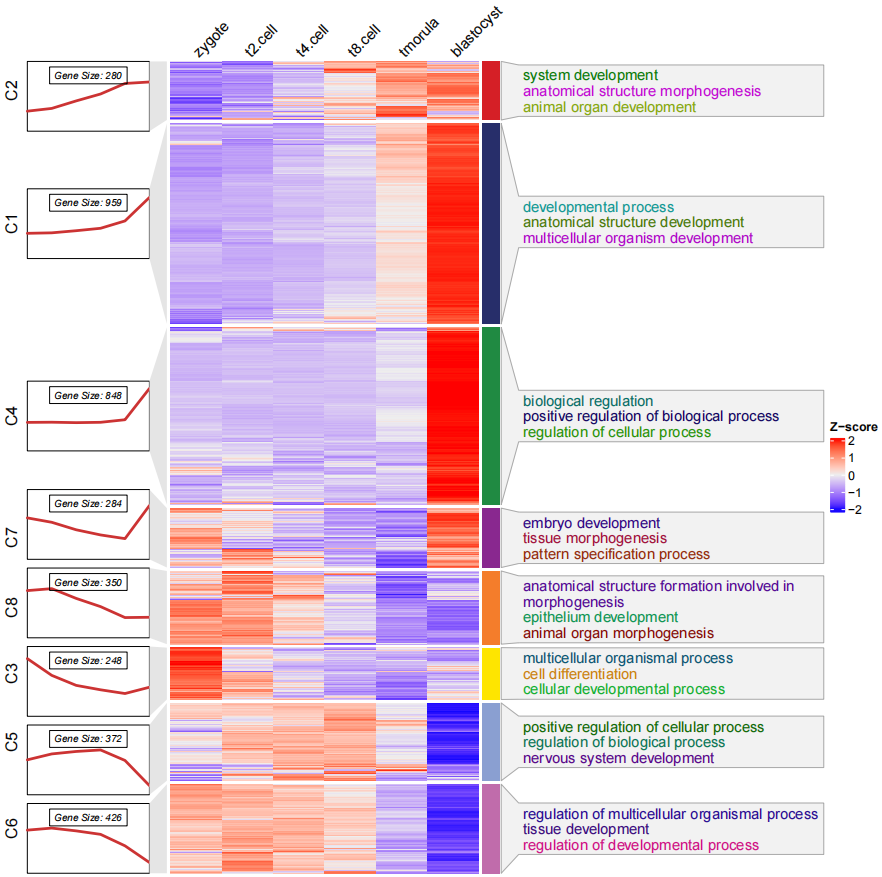
有任何疑问和想法,欢迎在 github 上面交流讨论!