Home
Binary Viewer is a tool for binary file discovery using visualizations that may highlight patterns.
Files are loaded by selecting the Load File button. One can select as many files as desired and then step through then using the Prev and Next buttons.
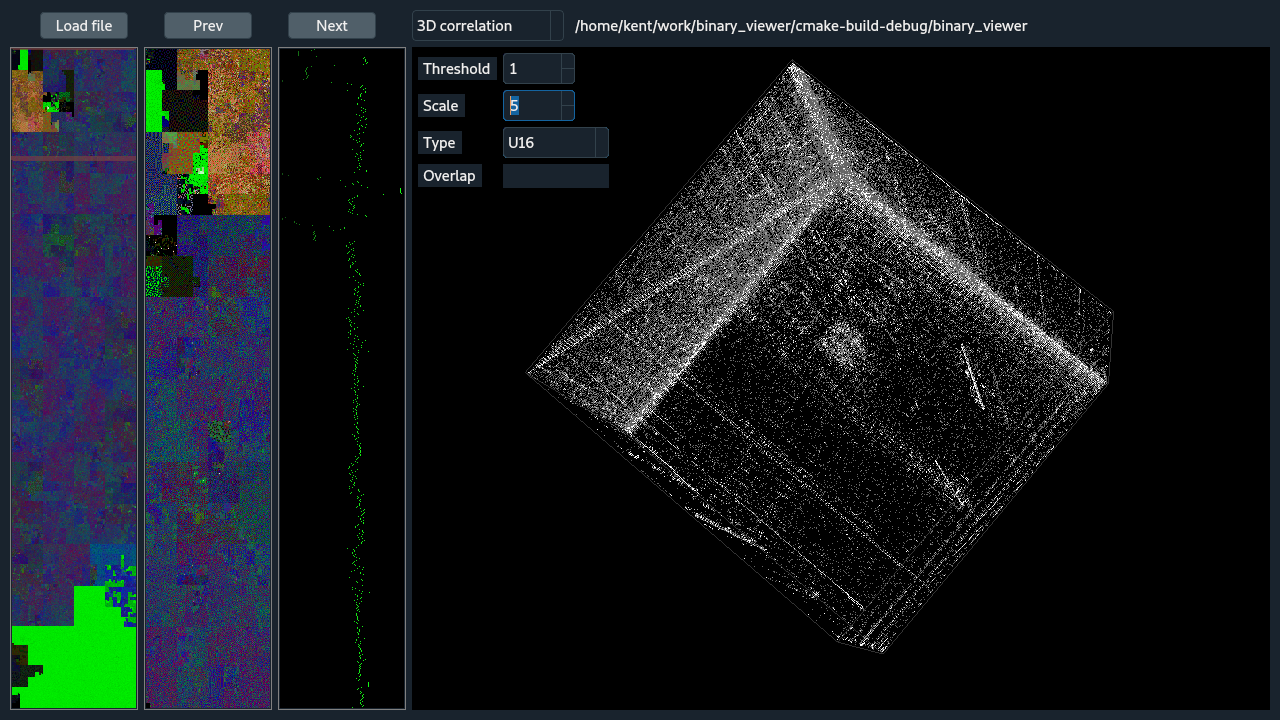
The screen is divided into three columns on the left and one large viewing region on the right. The the columns give, left to right, an overall view of a binary, an overview of the zoomed in region, and a stats view of the zoomed in region.
The overall and zoomed overviews represent the values and order of the bytes in the file, scaled to fit the region. Small files may have each byte represented by multiple pixels and non-overlapping chunks of bytes in large files may be represented by single pixels. The views have four modes which are Hilbert curve (on or off) and byte class highlighting (on or off). To cycle through the modes, click with the right mouse button. When byte class highlighting is on, bytes are colored by the class of byte (0, low bytes, ascii, high values, 0xff) otherwise bytes are colored by the byte value. For chunks, the color of the byte classes or the byte values will be averaged. Bytes are eithe rarranged linearlly, left or right top to bottom, or displayed on a Hilbert curve, similar to Conti's online viewer. The advantages of the space filling Hilbert curve is that bytes are are close in the linear file dimension tend to remain close on the 2D representation. When viewed linearlly, there is an arbitrary chunking created by the view width. Zoom is done by dragging the borders from the top and bottom of the left-most column, which start at the extremes of the binary. Once boundaries are selected, the region can be dragged. Other than the overall view, all other views depend on the selected region.
The stats column have two views: entropy and a histogram of byte values. The entropy view may help to find encrypted or compressed regions. The two views are toggled by right clicking on the stats column.
The main view is controlled with the pulldown above it. Next to the pulldown is displayed the path of the currently displayed file. The main views are: 3d histogram, 2d histogram, hex-text view, image view, and dot plot.
The 3d histogram shows in a 3D cube the frequency of neighboring 3-tuples, which are optionally overlapping. The spinning of the cube can be paused by clicking the cube with the right mouse button. The cube cannot be orientated with the mouse. The options are: Threshold is the minimum count needed before a tuple will be shown and can be used to reduce the noise. Scale is used to normalize the counts and can be used to ignore excessively frequent tuples by crushing the counts of the most frequent tuples. Type gives a means to change the datatype that the binary will be casted to for analysis. And Overlap allows byte-wise overlap of the data which may help in the case of frame-shifts.
The 2D histogram view is similar to the 3d version, the obvious difference being the histogram is computed with 2-tuples. The descriptions of the shared options are identical to the 3D histogram view.

The hex view shows hex and ASCII values of the file divided by rows of 16 bytes. The hex values are color coded based on byte class, similiar to the color codes used in the overviews. The entire file is accessible in this view and can be scrolled through with scrollbar, arrow keys, mouse wheel, etc. The start of the view is updated with the zoomed region. In the ASCII display, a small dark '.' is used for unprintable characters.

The image view interprets the zoomed region to be a raw image with the selected pixel count width. Various pixel formats are available including gray, RGB, and Bayer in various bit depths. The Offset is used to align the columns of the image.

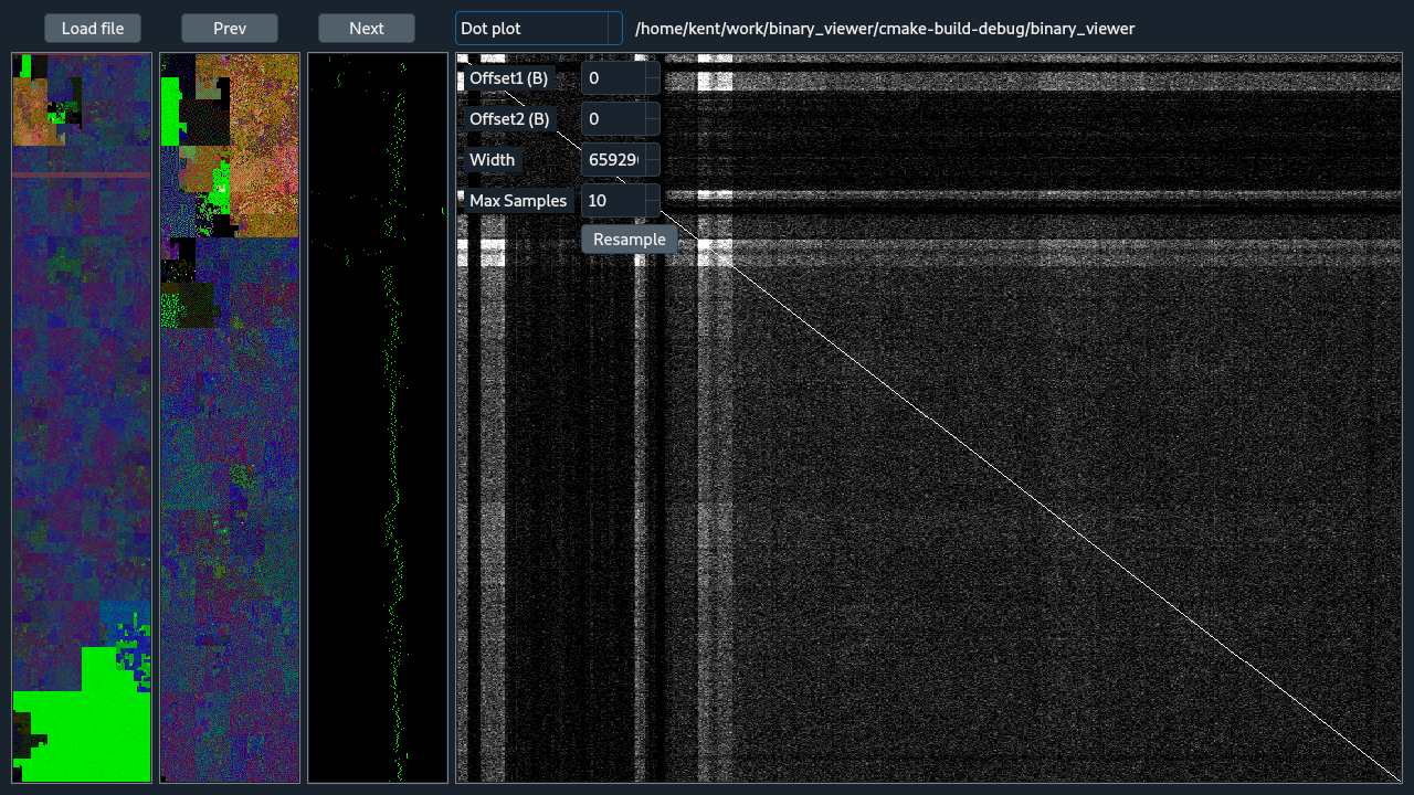
The dot plot view is shows a 2D self correlation, comparing the zoom region with itself. This is useful for finding duplication, reversals, and other similarities at potentially arbitrary distances. To start with, the two Offset values will be 0 which aligns the view along the main diagonal. The main diagonal will always be bright because pixels along the diagonal represent the comparison of the binary with itself without any shift, a perfect match. Adjusting the Offset values fine tunes the what has been selected with zooming, and moves the dot-plot analyzed region away from the main diagonal. The dot-plot is an O(n^2) comparison and for large files is impractical to compute, store, and display. So, to make the operation more suitable for large files the binary is broken up into non-overlapping blocks that depend on the binary size and the display size. Then sampling of the block-size^2 region is done emphasizing the diagonal of the block. Traditional dot-plots from genomics would not do this because it has a tendency to reduce highlighting reversals but reversal do still appear, they are dim, and it's not expected that reversals are too common. The number of samples is controlled by the Max Samples parameter, where that many samples are taken of the block diagonal and then again off diagonal. Within a block, where pixel of the final dot-plot has a block, an comparison of identity is done between each of the sampled points. The number of sampled pairs of points that are identical between becomes the value for that point in the dot plot. After all the comparisons are complete, the dot-plot is scaled for viewing. The Resample button repeats the sampling and analysis and should be selected a few times to test the robustness of the dot-plot.
Loosely based on Cantor.Dust, Binary Viewer was developed after seeing a demo of Cantor.Dust but receiving no response regarding availability.
Since Cantor.Dust was demoed, other tools with have similar functionality became available.
https://github.com/devttys0/binwalk/wiki/Quick-Start-Guide https://sites.google.com/site/xxcantorxdustxx/home
https://github.com/wapiflapi/binglide
https://github.com/codilime/veles
https://github.com/radareorg/radare2
The beginnings of Cantor.Dust was Greg Conti's work
https://github.com/rebelbot/binvis
Even earlier are dotplots for RE'ing, here Dan Kaminsky's Blackops talk https://www.slideshare.net/dakami/dmk-blackops2006
For more information on this and related programs for visualizing binaries see https://www.youtube.com/watch?v=C8--cXwuuFQ&list=PLUyyOw61zxiJXMihb4PjYbGHEgdGxMuY3
Qt5 is required to compile Binary Viewer.
Kent A. Vander Velden kent.vandervelden@gmail.com