2a. Intracranial EEG preprocessing
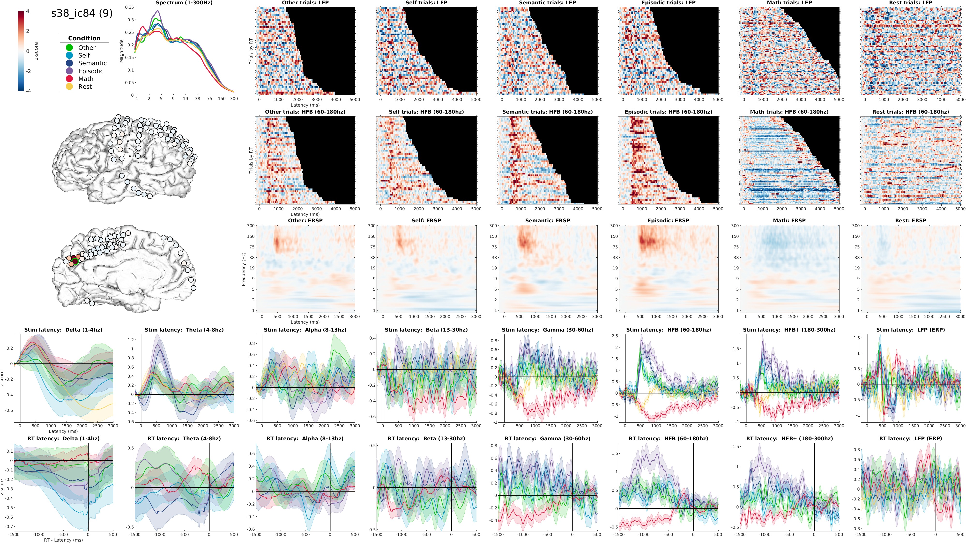
Summary statistics of an independent neuronal source decomposed by electroCUDA
This pipeline centers around artifact subspace reconstruction (ASR) and independent components analysis (ICA), a complementary combination of non-stationary & stationary decomposition that dramatically improves SNR & source separation (7~13db). This pipeline is compute-intensive but significantly improves data quality relative to standard pipelines.
The following pipeline and suggestions are based on my experience with mixed ECoG/sEEG data (100+ subjects from Stanford Medical Center & Beijing Neurological Institute)... Hope to do mass-scale empirical testing of denoising efficacy, send data!
Anatomical preprocessing follows the Freesurfer-based iELVis pipeline with modifications for feature enhancements & compute optimizations.
- Reconstruct & segment anatomical MRI into native & standardized cortical surfaces [all performed on Freesurfer; no electroCUDA code]
- Localize electrode position coordinates, correct post-implantation drift & align to cortical vertices:
~/src/anatomy/dykstraElecPjct.m - Calculate electrode anatomical attributes (proximal tissue density, etc) & parcellate into standard brain atlases (HCP-Glasser, Yeo networks, etc):
~/src/anatomy/ec_mkSubjVar.m - Aggregate all electrode metadata for further analyses:
~/src/anatomy/ec_mkChNfo.m
All preprocessing is performed on continuous timecourses, with many routines performed within-run to avoid edge artifacts (critical for filtering & time-frequency decomposition).
- Main function:
~/src/signal/ec_preproc_iEEG.m
- Load raw iEEG data.
- Identify irredeemably bad channels (empty, loose contact, etc) – check clinician/experimenter notes & enter known irredeemable chans to guide heuristics
- Identify remaining 'bad' channels with the ImaGIN classifier & other heuristics
- Robust detrend within-run to remove slow drifts (DC/impedance/etc). This fits lower-order polynomials on time windows, then fits higher-order polynomials to entire run. Noisy timepoints are updated per iteration & excluded from model fitting.
- Robust reference all channels to the iterative mean of remaining 'good' channels. Rank correction is applied if previous referencing is detected (most amplifiers reference during recording) or when 'bad' channels are excluded from reference calculation.
- Remove powerline noise with Zapline Plus. This uses adaptive heuristics to subtract PCA components with high powerline noise (50hz or 60hz depending on recording location) across overlapping time windows. In my experience this works best after detrending & referencing but before ASR.
- Remove non-stationary noise with ASR. This uses adaptive heuristics to subtract 'noisy' PCA components across overlapping sliding windows. Heuristics find the 'cleanest' section of the recording for iterative classification of 'noisy' PCA components across overlapping sliding windows (using Euclidian or Riemannian distance). In my experience, ASR works best after detrending, referencing & powerline denoising. However, ASR is often used as the first preprocessing step.
- Main function:
~/src/signal/ec_preprocICA.m
Independent components analysis (ICA) isolates unique sources of neuronal activity & noise (e.g. EMG/EKG/ocular/powerline). ICA transforms multichannel data into independent components (ICs): constituent sources of the recorded signal. Neurogenic ICs should be maximally independent of each other & any noise sources. In my experience, most neurogenic iEEG ICs are highly focal (<10 mm width) with occasional 'network-like' cross-regional ICs. Artifactual ICs tend to be localized to known bad channel(s) or specific electrode arrays (e.g. grid-specific noise).
- Prepare data for ICA using all redeemable channels. If rank deficiency is detected, dimensionality reduction is performed using channel exclusion or PCA. Heuristics calculate rank-deficiency contribution via leave-one-channel-out permutations, which determines required channel exclusions among 'bad' channels. If not rank sufficient after excluding all 'bad' channels, all redeemable channels are kept & PCA is performed instead. Note: PCA can worsen ICA decomposition so channel exclusion is preferred if only 'bad' channels need excluding. Otherwise, PCA is preferred to maximize data.
- Run ICA on the rank-sufficient data (dimensionality can't exceed rank). Besides the prior step, don't exclude 'bad' but redeemable channels as they improve noise decomposition.
- Reconstruct IC timecourses by applying ICA transformation matrices to channel data. IC indices are ordered from highest-to-lowest variance. IC names reflect highest-correlated iEEG channel (out of entire montage with no repetitions). You now have two datasets: channel data and IC data.
- Identify bad ICs with ImaGIN. Modified heuristics use classifier results, bad signal metrics (hurst exponent/kurtosis/variance-covariance) & correlation/covariance with known irredeemable channels.
- Denoise channel data by subtracting 'bad' ICs via backprojection. If only performing channel-space analyses, IC data can be deleted upon completion. If only performing IC-space analyses, this step can be skipped since neurogenic ICs are already isolated from 'bad' ICs. The suffix "c" is appended in filenames after subtraction; non-subtracted data are saved without suffix (see Filestructure).
- Main function:
~/src/signal/ec_preprocTimeFreq.m
Continuous wavelet transform with Morse wavelets are used by default, as they account for unequal variance-covariance across frequencies. L1-norm is applied to mitigate the 1/frequency decay of neuronal field potentials. Wavelet transforms are performed within-run to avoid edge artifacts.
- Load denoised dataset(s) & perform continuous wavelet transform for a desired frequency range. This generates individual timecourses per frequency (spectral multi-frequency) or mean timecourses within the frequency range (repeat for each desired spectral band)
- Identify remaining noisy timepoints (spikes, pops, channel-specific artifacts, etc) within each band/frequency per channel/IC... Choose whether to keep, interpolate or remove these timepoints in later analyses.
Optional steps for gamma or HFB bands
- Main functions:
~/src/signal/ec_preprocTimeFreq.m&~/src/signal/ec_preprocICA.m
ICA on full-spectrum recordings (step 9) can be biased towards lower frequencies due to the 1/frequency decay of neuronal field potentials, which reduces variance at higher frequencies. Thus, lower-frequency activity (mostly delta, theta & alpha) can have greatest influence on ICA decomposition. Re-running ICA on high-freq timecourses may result in better decomposition of high-frequency neural & noise sources
- Rerun ICA using channel timecourses of HFB or gamma activity. Ensure that input channel data have NOT undergone subtraction of 'bad' ICs to avoid rank deficiency (i.e. Step 12, non-subtracted data are saved without suffix "c"). Full-spectrum ICA weights (from Step 9) are used as initial weights. This optimizes ICs for HFB/gamma dynamics without wasting the full-spectrum decomposition.
- Using high-freq ICA, identify 'bad' ICs & subtract from HFB/gamma channel data (step 11-12 for HFB/gamma only)
- Identify remaining noisy timepoints (spikes, pops, channel-specific artifacts, etc) in HFB/gamma per channel/IC... Choose whether to keep, interpolate or remove these timepoints in later analyses (step 14 for HFB/gamma only).