changed Buildings.Fluid.Movers.BaseClasses.Characteristics.power: #202
Conversation
|
Should I have added author information? Please let me know if I need to change things :) Filip |
|
Is there a physical rationale for the change
If there is really a dependency on Note that |
|
Yes there is a physical rationale for this change. Allow me to (try to) explain based on this figure: Similarity laws hold for two similar working points. Consider state 1 (nominal speed) and state 2. For these states the following equations hold: So in the code the last equation is used. For this equation to hold you must evaluate P1 based on its working points q1 and dp1 as if it were running at nominal speed. Right now you use q2 te evaluate P1, which should be q1 = q2/r_N. You can see this also from the figure where the different working points have different mass flow rates. Another way to show this: The way my adjustment works is to evaluate the polynomial as if it were running at the rotational speed for which it was constructed and then transforms the result to the correct rotational speed. Note that for similar working points the efficiency is the same (see above) and therefor using a term such as eff(r_N) does not really make sense to me. I did not check with different manufacturers but I did check for two different types and three different sizes of pumps. I also have a fourth example where similarity laws somehow do not seem to hold (regardless of the adjustment): Regarding your last comment: |


|
I agree with this change and will merge it to the master. |
|
Filip, can you please add an example in |
|
woops, deleting branches causes problems here.. Unfortunately you cannot exactly generate the graphs from the file I added. I use a Python script for this myself. Plotting output_y should however give close results. |
|
Thanks for the updated pull request. I am revising the code, but most Michael On Thu, Feb 27, 2014 at 4:01 AM, Filip notifications@github.com wrote:
|
This is for #202. Minor changes in reference results. Also updated YorkCalc.mo which also uses the efficiency function.
|
Hi @mwetter I think that the problem described above for FlowMachine_Nrpm also applies to FlowMachine_m_flow and FlowMachine_dp. Right now the efficiency/power is calculated based only on r_V, the pump speed is not taken into account. In think N should first be calculated from m_flow and dp. From this N, r_N can then be calculated and this would allow to calculate the efficiency in a way similar to FlowMachine_Nrpm. I overlooked this in ibpsa/modelica-ibpsa#56 but better late than never.. Fixing this may however prove difficult since N needs do be calculated from the discretised relation V_flow = f(dp) and the similarity law equations. Filip |
|
This has been merged to the development branch lbl-srg:issue209_pumpRecords rather than the master, see #285. @Mathadon : can you please explain what the problem is with "Right now the efficiency/power is calculated based only on r_V, the pump speed is not taken into account." Do you suggest to redefine the signature of the motor and hydraulic efficiency functions? If so, how do you propose them? |
|
A more elaborate explanation: In this case we have eta1 = f1(r_V1) for n = n1 (the nominal curve) and f1 known Since f2 is unknown we would like to use eta1 = eta2 = f1(r_V1). This is only valid if the two working points are similar so we also require: furthermore we have: we know n1 (nominal rpm), q2 (mass flow rate setpoint), dp2 (from load), so unknowns are n2, q1 and dp1. They can be solved from equations 1,2,3. Knowing q1, then r_V1 can be calculated and from this eta1= eta2 = f1(r_V1). The power can be calculated in a similar way. I am however unsure of how to solve this using the existing 'piecewise' functions but it may be sufficient to plug the above equations in Modelica. Note that this complicated system does not need to be solved in pump_Nrpm since there you explicitly set n2, which simplifies things. Fyi: I have been working on a pump model that explicitly contains equations 1, 2, 3 where equation 3 is a polynomial but numerically it can be quite difficult to solve. I managed to improve this a bit by using n2 as a state, which corresponds to a physical impeller inertia but introduces a small time constant. Let me know if this is of interest? Kind regards! Filip |
|
@Mathadon : I suggest you write up on 1 or 2 pages what changes you specifically propose, and propose an example implementation. The explanation above is quite confusing and I would have to speculate what you mean, rather than clearly understand what the change proposal is. Inverting a polynomial is something we rather don't do unless we know for sure (i.e., can prove) that there is only one solution. Otherwise, the solver will fail in some situations. Also, adding a fast transient is not desirable as |
This is for lbl-srg#202.

Conflicts:
	Buildings/Fluid/Movers/BaseClasses/Characteristics.mo
	Buildings/package.mo
|
According to me, the reasoning of Filip is right. However, the solver will need to solve a set of non-linear equations including the polynomial. Some investigations of the uniqueness of the solution should be done. |
Hi,
I made the following changes:
Similarity law now uses a working point based on a rotational speed V_flow/r_N instead of V_flow. Only when referring to this working point then the power law P2= r_N^3*P1 is valid.
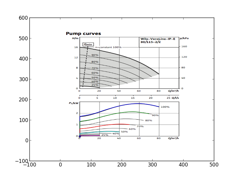
I have some images that can serve as a limited validation. The graphs you see are from the data sheets from real pumps.


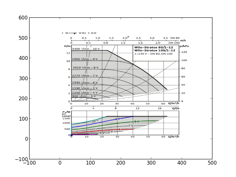


Before:
After:
Also, for the following figures I changed the power law from:
P:=r_N^3_Buildings.Utili ....
to
P:=r_N^2.75_Buildings.Utili ....
This seems to give even better results:


Although not related to the similarity laws, this behavior can be explained by the fact the electrical motors usually become more efficient for higher powers and that this is not reflected in the power law. Is there a way this can be implemented in the buildings library as well?
Kind regards,
Filip