Hybrid sort
Quicksort decrease efficiency when N becomes small as below. The following table exhibits the rate of division in partitioning.
$ N=10000; src/random.awk $N | Debug/Sort -N $N -rP 31,127,4095,0 -D 3 -V 2 |
> src/rate.awk | expand -t 5
quick_random()
     0.0  0.1  0.2  0.3  0.4  0.5  0.6  0.7  0.8  0.9  1
00   1349                                              345
01   554            137       276       158            235
02   328  26   91   126  91   117  99   73   174  27   119
03   127  72   72   99   70   91   88   57   92   97   50
04   56   57   40   48   59   58   54   48   56   47   30
05   2    15   25   29   35   38   39   27   24   16   2
06   2    3    11   15   23   24   16   21   11   5    2
07        3    4    9    9    15   12   6    4    2
08                  4    5    7    5    2    2    1
09             1    2    2    4    4    2    2
10        1         3    1    1         2
11                  2    1    1
12                                 1    1
13                            1
While N is large, the rate gathers to the center by the choice of median.
However, when N becomes small, the rate spreads.
I suggest to switch algorithm from quicksort to indirect
mergesort
when N becomes small.
Mergesort takes 2 advantages over quicksort:
The number of comparison is less than quicksort,
and the fall of performance against the worst data is small.
On the contrary, Mergesort takes 2 disadvantages over quicksort:
The number of copies is more than quicksort,
and simple Mergesort requires more memory than quicksort.
However, these disadvantages are reduced by indirect Mergesort when N is small.
Simple Mergesort divides an array to 2 half sub-arrays recursively until a sub-array contains 1 element,
then merges back divided two sub-arrays choosing lesser element of them iteratively.
As a result, the merged array is sorted.
Simple Mergesort duplicates
source array and uses them alternately as below,
thus Mergesort requires large memory if N or a size of element is large.
A : (c, d, b, a)      Source array A.

A : (c, d, b, a)      Duplicate and divide A to B.
B : (c, d), (b, a)

A : (c), (d), (b, a)
B : (c, d), (b, a)    Divide (c, d) in B to A.

A : (c), (d), (b, a)  Move (c) in A to B,
B : (c, d), (b, a)    append (d) in A to B.

A : (-, -), (b), (a)
B : (c, d), (b, a)    Divide (b, a) in B to A.

A : (-, -), (b), (a)  Move (a) in A to B,
B : (c, d), (a, b)    append (b) in A to B.

A : (-, -, -, -)      Move (a) in B to A,
B : (c, d), (a, b)    append (b), (c, d) in B to A.

A : (a, b, c, d)      Discard B.
The numbers of times are computable for the both best and worst case in Mergesort.
Sorted data is the best case for Mergesort,
because in merging,
when a lesser sub-array empties,
another greater sub-array appends to the copied array without comparison,
thus the number of comparison is the least.
$ N=16384; src/sorted.awk $N | Debug/Sort -N $N -mV 1
arguments : -N 16384 -mV 1
qsort(3)     usec = 5311 call = 0     compare = 114688 copy = 0
merge_sort() usec = 3524 call = 16383 compare = 114688 copy = 131071
merge_sort : Mergesort called by -m option.
If N=2^k then the depth of call is k,
and N/2 elements are compared in each depth,
thus the number of comparison is Nlog2(N)/2:
16384*14/2=16384*7=114688.
The number of calls is N-1,
because every recursive call inserts a gap between 2 sub-arrays,
and finally a source array is divided into individual elements
and N-1 gaps are inserted.
The number of copies is added number of calls and comparisons,
because when a lesser sub-array empties,
a greater sub-array appends to the lesser sub-array by block-copy without comparison:
16383+114688=131071.
On the contrary in the worst case,
only one element is left in a sub-array when another sub-array empties.
The following list exhibits the worst case for Mergesort.
$ src/merge.pl 8 | xargs echo   # example
7 3 5 1 6 2 4 0
$ N=16384; src/merge.pl $N | Debug/Sort -N $N -mV 1
arguments : -N 16384 -mV 1
qsort(3)     usec = 9049 call = 0     compare = 212993 copy = 0
merge_sort() usec = 6696 call = 16383 compare = 212993 copy = 229376
merge.pl : perl script to generate data sequence to maximize the number of comparisons for Mergesort.
N elements are copied in each depth, thus the number of copies is Nlog2(N): 16384*14=229376. The number of comparisons is attracted calls from copies:229376-16383=212993.
The following list exhibits the case of random data.
$ N=16384; src/random.awk $N | Debug/Sort -N $N -mrP 31,127,4095,0 -V 1
arguments : -N 16384 -mrP 31,127,4095,0 -V 1
qsort(3)       usec = 14136 call = 0     compare = 208792 copy = 0
merge_sort()   usec = 7948  call = 16383 compare = 208792 copy = 225175
quick_random() usec = 8485  call = 10267 compare = 232310 copy = 127709
In merge_sort(),
the number of comparisons and copies are not so different from the worst case.
Therefore in the worst case, the fall of performance is small from random data.
The number of comparison in merge_sort() is about 10% less than in quick_random().
However the number of copies in merge_sort() is more than in quick_random(),
because it is greater than the number of comparison in Mergesort,
thus it is not so different from the number of comparisons in quick_random().
On the contrary in quicksort,
the probability of copy after comparison is 0.5.
Therefore the number of copies in Mergesort is about 2 times of it in quicksort.
This is the reason why quicksort is faster than Mergesort usually.
Nevertheless, the number of copies in Mergesort is reduced by indirect sort, and work-space is not large when N is small. Quicksort is efficient when N is large, thus quicksort and indirect mergesort are complemental to each other.
$ N=100000; src/random.awk $N |
> Debug/Sort -N $N -mrP 31,127,4095,0 -D 3 -L 1024 -qA M -V 1
arguments : -N 100000 -mrP 31,127,4095,0 -D 3 -L 1024 -qA M -V 1
qsort(3)       usec = 54578 call = 0     compare = 1536283 copy = 0
merge_sort()   usec = 62532 call = 99999 compare = 1536283 copy = 1636282
quick_random() usec = 56981 call = 62920 compare = 1693133 copy = 907247
quick_hybrid() usec = 53483 call = 99846 compare = 1604344 copy = 448759
quick_hybrid : Hybrid sort of quicksort called by -q option.
Indirect Mergesort is called by -A M option when N becomes small.
quick_hybrid() begins with quicksort and changed to indirect Mergesort when N<=1024 by -L option.
The number of comparisons in quick_hybrid() is less than quick_random() and more than merge_sort().
The number of copies in quick_hybrid() is the least.
The following chart exhibits the relative elapsed time in various threshold to change algorithm.
Y axis is normalized elapsed time / nlog(n),
where the average of quick_hole() is 1.
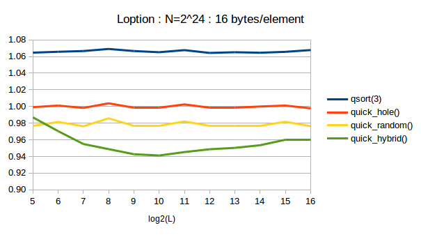
Data.
I determined the threshold to 1024.
The following chart exhibits the relative elapsed time in various N.
Y axis is normalized elapsed time / nlog(n),
where the value of quick_hole() at N=2^20=1M is 1.
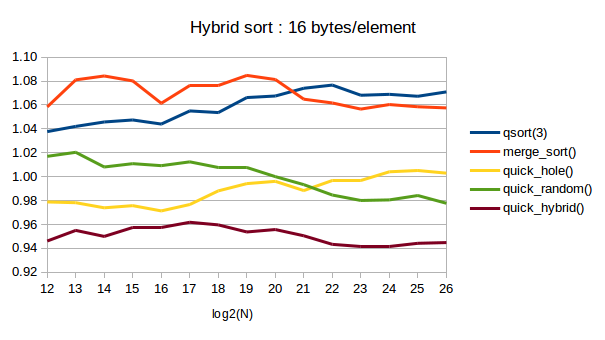
Data.
quick_hybrid() is the fastest.
[Up] : Home
[Prev] : Indirect sort
[Next] : QMI-sort