FIN 5624 - Numerical Methods - Fall 2014

The course examines numerical methods for valuing financial derivatives. Topics include:

• Tree Methods
• Finite Difference Techniques
• Financial Engineering Methods and MATLAB

October 21 Exam

Asian option with geometric average:

>> GeoCall(30,30,.07,.01,.30,1)

ans =

	2.2870

2D Plot

Asian option with geometric average:

3D Plot

Asian option with geometric average:

October 14 Assignment

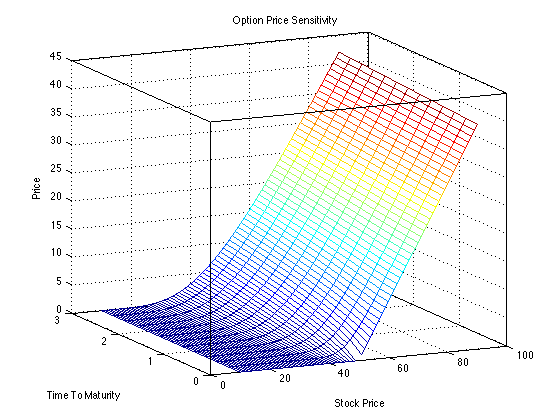
>> BlackScholes(50,50,1,.05,.2,0.02,1,0)

Price

ans =

	4.6135

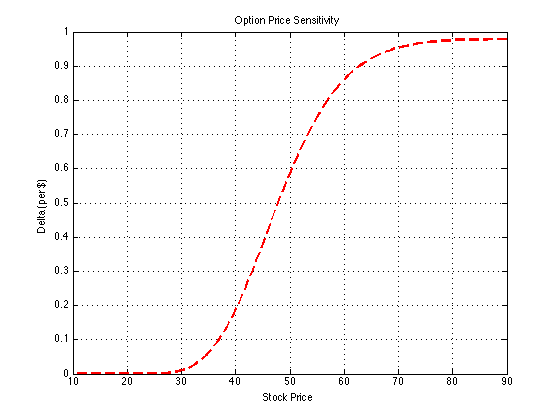
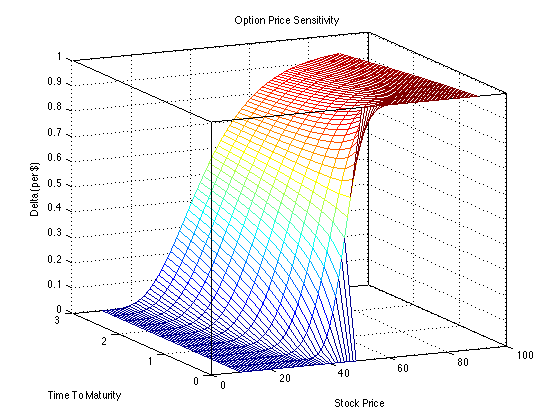
>> BlackScholes(50,50,1,.05,.2,0.02,1,1)

Delta

ans =

	0.5869

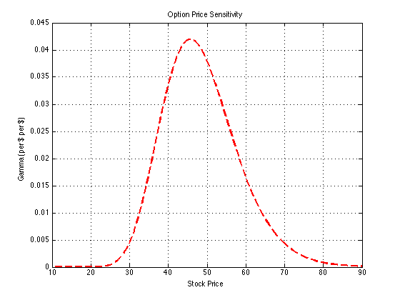
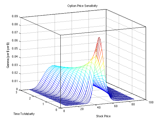
>> BlackScholes(50,50,1,.05,.2,0.02,1,2)

Gamma

ans =

	0.0379

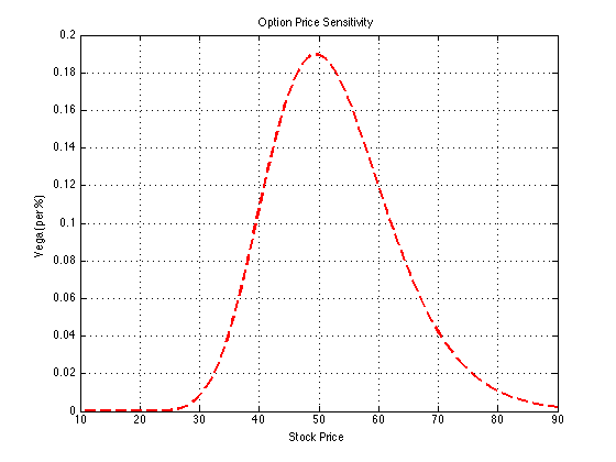
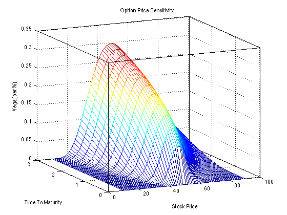
>> BlackScholes(50,50,1,.05,.2,0.02,1,3)

Vega

ans =

	0.1895

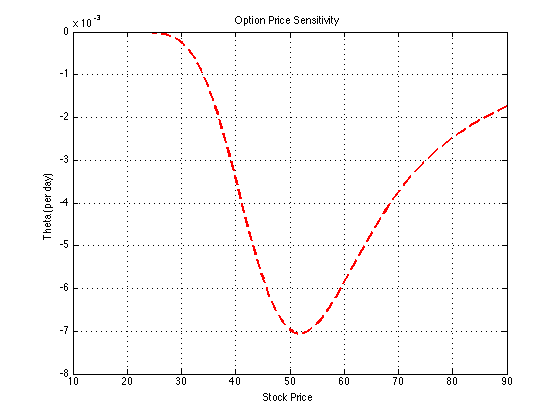
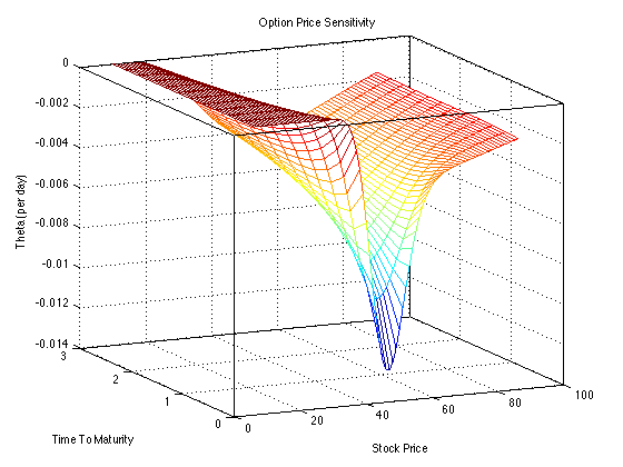
>> BlackScholes(50,50,1,.05,.2,0.02,1,4)

Theta

ans =

   -0.0070

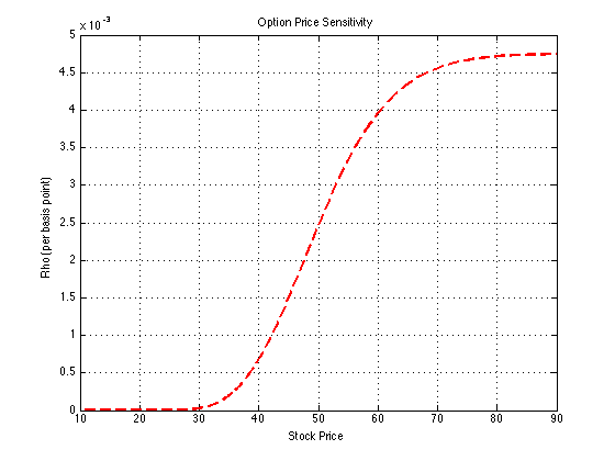
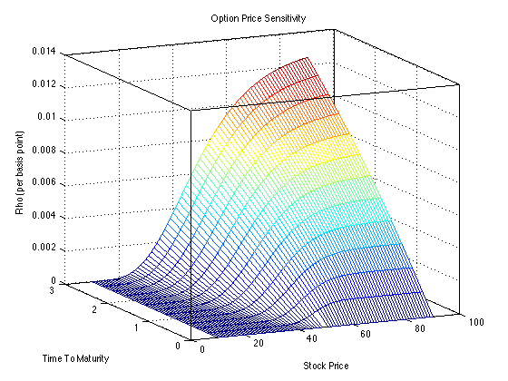
>> BlackScholes(50,50,1,.05,.2,0.02,1,5)

Rho

ans =

	0.0025

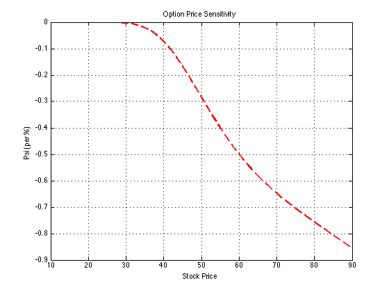
>> BlackScholes(50,50,1,.05,.2,0.02,1,6)

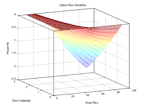
Psi

ans =

   -0.2848

>> BlackScholes(50,50,1,.05,4.6135,0.02,1,7)

Implied Volatility

ans =

	0.2000

>> BSImpliedVol_Newton(50,50,1,.05,4.6135,0.02,1)

Implied Volatility (Newton's Method)

ans =

	0.2000

2D Plots

3D Plots

October 7 Assignment

BSCall.m

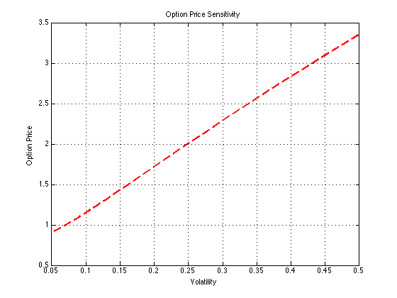
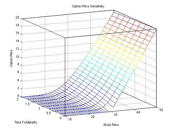
Write a function BSCall(S, K, r, q, vol, T) that returns the BlackScholes price of a call.

>> BSCall(50,50,.04,.017,.20,1);
4.4555

BSPut.m

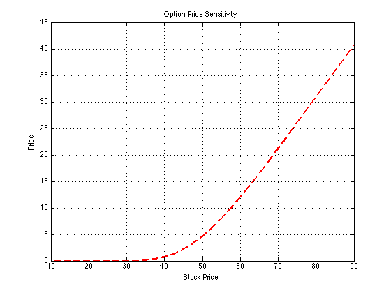
Write a function BSPut(S, K, r, q, vol, T) that returns the BlackScholes price of a put.

>> BSPut(50,50,.04,.017,.20,1);
3.3378

BSCall_plot.m

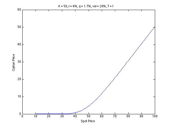
Write a script function that plots the price of a European call versus the Stock price S given K = 50, r = 4%, q = 1.7%, vol = 20%, T =1.