PE-ratio-and-stock-return-analysis

---

Step 1: download the pe ratio from the choice database

In this step, the first thing we have to notice is that the structure from the choice database is cross-sectional dataframe.

Therefore, in order to get the exact data in a certain time point, we need to get the list of trade date (from the tushare database), so that we can wedge these date into our codes.

Specifically, I will select several time span to do this research, which is because we can use the different period of testing result to explain the relationship between P/E ratio and holding stock return in a specific time period. Further more, if the result of the testing is correspondent to what we expect in the beginning, then we can use the result to describe the current situation of the underlying asset for its future prospect.

In order to make this research correspond to the recent circumstance, the period that we select is from 2012 to 2018.

Step 2: download the open and close stock price from the tushare database

We have discussed the procedure of doing the research in above discription, which we should get the trading date firstly. Here we can directly select a period, which does not need to be the exact trading date. Then this trading date could be used to be the paramater to download the data of P/E ratio.

ts.get_k_data('000300', index=True,start='2017-06-30', end='2018-01-01').date

Meanwhile, we can also get the data of open and close stock price.

ts.get_k_data('000300', index=True,start='2017-06-30', end='2018-06-30')

After we get the trading data, the next step is to calculate the accumulative return for the correspondent P/E ratio. We are going to discuss deeply the logic of how the length of time series be selected.

ret = np.zeros(125)
n1, = ret.shape
rt = np.array(price2['close']/price2['open'])
n2, = rt.shape
for j in range(n1):
  ct = rt[0]
  for k in range(1,125):
      rn = rt[j+k]
      ct = ct * rn
  ret[j] = ct - 1

Step 3: run the regression model and interpret the result

First of all, the regression model that we construct is:

where:

From the equation, we know that the the correspondent Y_T is the holding rate of return (from time t to T) after we bought in the asset as we observed the P/E ratio in time t.

	return_6m	return_1y	return_3y
HS300.index
const	2.1868	0.8299	3.0118
P/E coef	-0.1349	-0.0330	-0.1232
P value	0.000	0.000	0.000
R squared	0.786	0.115	0.456

Step 4: based on our observation and testing result, give our perspective on the underlying asset which we'd like to interpret its current position in the market

As we can see from the first figure in the following, the P/E ratio was climing from 2017/7/4 to 2017/12/29, and the holding rate of return for six month was decreasing as the same period.

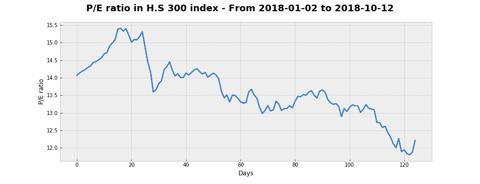
However, the P/E ratio was goling in the opposite way from 2018/1/2 to 2018/10/12.

As a result, we can conservatively assume that the current P/E ratio is in the relatively low position comparing to the past six month.

Reference

[1] Liem, Pei Fun, and Sautma Ronni Basana. "Price Earnings Ratio and Stock Return Analysis (Evidence from Liquidity 45 Stocks Listed in Indonesia Stock Exchange)." Jurnal Manajemen dan Kewirausahaan 14.1 (2012): 7-12.
[2] Norbert Keimling. “PREDICTING STOCK MARKET RETURNS USING THE SHILLER CAPE.” StarCapital Research, January 2016.