This project introduces an architecture that optimizes Stencil Kernel Calculations and is offloaded to FPGAs with the use of Vitis (Vivado) High Level Synthesis tool (HLS).
Project is created with:
- C/C++
- Vitis HLS 2021.2
- Run Vitis (or Vivado) HLS adding the source & header files from the corresponding folder.
- The no. of Time-Steps is denoted as D.
- Each folder contains a version of the architecture with different Time-Step factors D.
- The DCMI_Jacobi.cpp file should be used as the top function for the implementation of a single time-step.
- Utilize the provided Test-Bench from the corresponding folder.
- In the header file the defined size of the grid can be modified.
The architecture proposed in this section is greatly inspired by the work done in [1]. The proposed architecture of [1] performs stencil calculation over an arbitrary number of 𝐷 time-domain iterations. Essentially the design bypasses the calculation of intermediate time-steps and outputs results directly for the target 𝐷.
Most of the ISLs’ core computation is a first degree, i.e., linear, polynomial. Constant coefficients are multiplied with the data elements of the stencil pattern and the sum of these multiplications holds the resulting value. These mathematical operations, i.e., addition and multiplication, are characterized by the commutative and associative properties, as it follows, the computation of each term in the polynomial can be calculated independently. Moreover, it is evident that the coefficients of the polynomial across multiple iterations are only dependent on the stencil pattern and the depth of the iterations therefore their calculation need not happen at runtime because the effective coefficients for every element can be computed beforehand, in design time.
An architecture tailored to suite the calculation of Jacobi 9-Point Stencil is proposed. The design utilizes the minimal amount of on-chip memory required to stream data and store them until all the resulting data that are dependent on it have been calculated. Each element is fetched once from external memory per accelerator invocation. The input and output of data transpires in a streaming manner and lexicographical order is maintained.

The abstract representation of the ICT Accelerator is provided in the Figure above. Considering one input, and depth 𝐷 the number of time-domain iterations for which we need a result, the design has been loaded with precomputed effective coefficients. The input is multiplied with the specific coefficients, depending on its iteration indexes, and the results are stored on the Reuse Buffer that holds the partial results. After the calculations are complete, the first element of the Reuse Buffer is outputted as a result and the buffer is shifted left.

The figure above, provides a naive example with the iteration depth 𝐷 = 1 and a small 2- dimensional grid of 4 ∗ 4. We examine the impact of the input data only in correlation with the element with the red color. For every new input, that is, the element colored in pink, the value of the input is multiplied with the corresponding coefficients, and the partial result is stored on the Reuse Buffer. This partial result describes how the pink element affects the red. It is referred to as partial because it makes up part of the total resulting value. On the next input, the next partial result is computed, and added to the previous one and so forth. Note that the Result Buffer shifts for every new input, so that the partial results are added to the correct elements in the buffer. The last element that needs to be read for the calculation of the data is shown in the final grid to the right. The partial result has been shifted to the left of the buffer. After the last partial result is accumulated with the rest, the calculation of the element in red is complete and it is fed to the output port.

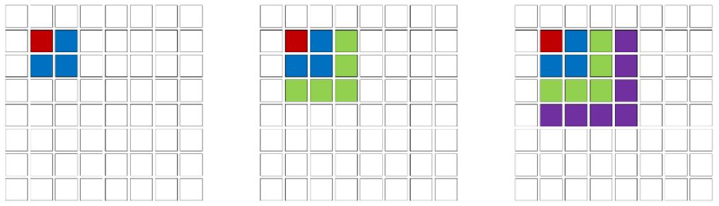
The nature of the precomputed coefficients requires further examination. Considering an arbitrary data element of a 2-dimensional grid, exemplified as the red square in the figure above, the elements that are affected by it, increase for every additional timestep. As portrayed, for a time-step equal to one (𝐷 = 1), figure (a) shows that the colored elements (red and blue) are affected by it, for two time-steps (𝐷 = 2) in figure (b), blue, green and the red elements are affected and so forth. Since the coefficient values are fixed, the design can identify the effective coefficients that are applied to each element from its neighboring ones after an arbitrary number of iterations. So this Figure, essentially shows how many values are affected by the red colored element for different values of 𝐷. The primary suggestion of [1] is that the effective coefficients, that describe how the red element affects each of its colored neighbors, can be computed before runtime.
The authors of [1] propose an algorithm to compute these coefficients. The algorithm determines the number of elements affected by a single input and creates an array of that size.
where 𝑅 denotes the radius of the stencil pattern. The radius of the stencil pattern is defined as the maximum iteration distance within the pattern, measured from the element at the center of the stencil. Regarding the 9-Point Jacobi kernel performing calculation over a 2-dimensional grid of size 𝐻𝐸𝐼𝐺𝐻𝑇 ∗ 𝑊𝐼𝐷𝑇𝐻, the radius is 𝑅 = 𝑊𝐼𝐷𝑇𝐻 + 1. 𝐷 denotes the time-step iteration depth.
Although the array size proposed by [1] withholds all the necessary effective coefficients, it lacks optimality in memory usage, since, depending on the stencil pattern, there might be array elements that remain zero after the computation. In the work of the present thesis, where square (9-Point) stencils are used throughout, the design choice was to optimize the size of the array as such:
This equation can be verified by the graphical representation of the above figure, as the colored elements follow that pattern of expansion with every increment of 𝐷.
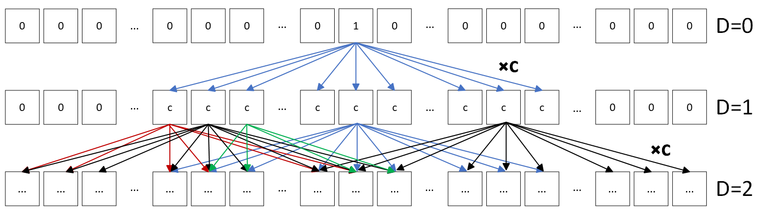
To create the array of effective coefficient, the following procedure takes place. The middle element of the array is set to one while the rest are set to zero. Then, the stencil pattern is applied to this input array over 𝐷 iterations. The resulting array holds the aggregate coefficient for each affected result value. The above figure provides an abstract representation of the described process, some interconnections as well as data elements have been omitted for simplicity and comprehension purposes. After the first iteration, the elements hold the original coefficients, denoted as 𝑐 in the graph. The arrows distribute and multiply data with coefficients according to the stencil pattern, and when two or more arrows have the same target, their values are summed. After the number of iterations has reached its goal, the array holds the combined coefficients of each result element.
An important aspect of calculating the Effective Coefficient Array is the edge case exceptions. The process described above, created an array that holds aggregate coefficients that can be applied to the intermediate data of an arbitrary grid. Whereas the same does not stand true for elements close to the edges. The figure above shows a differentiated expansion compared to the one of the previous figures. That is because of the intrinsic property of ISLs, that the halo data cannot be altered. Therefore, all elements in halo regions, and several others near them, require different effective coefficient arrays.
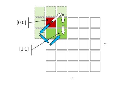
As described before, the effective coefficient arrays explain the way one element affects nearby ones, after some time-steps. The above figure provides a naive example of how the element of the grid [0,0], affects [1,1]. The arrows of this graph, have the same functionality as the ones in the figure before. Under normal circumstances, for the first timestep, the red element will affect the elements at the destination of the arrows, which exceed the limits of the grid, therefore they do not exist. These non-existent data elements will in turn affect halo elements, which cannot be altered. Finally, the arrows arrive in element [1,1] carrying partial effective coefficients that will be aggregated. The route of these arrows is invalid, as they describe ways that element [1,1] is affected by [0,0] which are not feasible.
The conclusion is therefore drawn, that for elements in the edges of the grid, different Effective Coefficient Array should be generated. To calculate the corresponding arrays of the elements near the edges, the same methodology as the intermediate ones is followed, albeit differentiating by restricting the effect of halo, or non-existent data. It arises, that with the incrementation of time-steps the design harvests parallelism from, i.e., the value of 𝐷, more Effective Coefficient Arrays need to be generated for the purposes of these edge case exceptions.

This figure presents the number of generated Effective Coefficient Arrays and their respective position on the four edges of the gird depending on the value of depth 𝐷. The squares marked with the same numbering utilize the same array. The white squares represent the intermediate ones, i.e., the ones calculated without any constraints. In the Figure (a), the design requires 25 distinct arrays, in (b) 49 and in (c) 81 are necessary. All these different coefficient arrays are pre-computed and stored on-chip, thus, are ready for use at run-time.
The design keeps two iteration indexes as it iterates through the 2-dimensional grid and decides which Effective Coefficient Array is corresponds to the data element that is currently processed. The input is then multiplied with the values in the array and the results are added to the partial results in the Reuse Buffer. That way all the possible result components from a single input value have been computed.
The Reuse Buffer stores these partially accumulated results. As described in [1] its size is:
Since we need to add multiple partial results to the Reuse Buffer, its memory elements need to be
structured in a way that allows for concurrent access, thus implementing the individual memory elements
as registers. Nevertheless, only

The data produced by the multiplication are in sets of 2 ∗ 𝐷 + 1. The number of these sets is again 2 ∗ 𝐷 + 1. Therefore, the Reuse Buffer is partitioned in 2 ∗ 𝐷 + 1 sets of 2 ∗ 𝐷 + 1 distinct registers. Between those registers, FIFOs are used to store the rest of the data elements, which do not participate in the accumulation. The above figure presents a simplified structure of the buffer. 2 ∗ 𝐷 + 1 sets of 2 ∗ 𝐷 + 1 data, have been created by the multiplication of the input value with the corresponding coefficients. Then they are accumulated with the already existent partial results and stored on the Reuse Buffer. The implementation of FIFOs in the areas of the buffer that do not participate in the accumulation, is cheaper than the use of individual registers and, saves the need for indexing data that would be needed to match the data destined for accumulation.
The Reuse Buffer outputs its left most element, portrayed in yellow in the Figure, as its calculation has been completed. Certainly, a delay in output introduced, which is proportional to the value of 𝐷 chosen. The delay is perfectly exemplified by the previous figures, for every different 𝐷 the input of the last colored element is requisite for the calculation of the middle one. Therefore, the delay is equal to:
Again, the design has an intrinsic latency measured from the clock cycle that the last necessary input is available, up to the clock cycle that the result is outputted. This intrinsic latency will be denoted as 𝐼𝐶𝑇𝐴_{𝐿𝑎𝑡𝑒𝑛𝑐𝑦}. Given that the stencil pattern slides through a grid of size 𝐻𝐸𝐼𝐺𝐻𝑇 ∗ 𝑊𝐼𝐷𝑇𝐻 ,the total latency of the design is provided by the equation bellow.
[1] Mostafa Koraei, Omid Fatemi, and Magnus Jahre. 2019. DCMI: A Scalable Strategy for Accelerating Iterative Stencil Loops on FPGAs. ACM Trans. Archit. Code Optim. 16, 4, Article 36 (December 2019), 24 pages. https://doi.org/10.1145/3352813