Grab AI's Computer Vision Challenge 2019

Introduction

This project is created as a submission for the Grab AI's Computer Vision Challenge 2019

Outcome

This is one of the top 50 best projects in the Grab AI Challenge 2019 (among 1200 participants):

Problem Statement

Given a dataset of distinct car images , can you automatically recognize the car model and make?

Installation

The code was written and tested on Ubuntu 16.04, and the following packages were used:

• Python 3.6.7
• OpenCV 4.0.0
• Numpy 1.16.2
• scikit-learn 0.20.3
• matplotlib 3.0.2
• Tensorflow 1.12.0
• Keras 2.2.4

Make sure you have these installed in order to run the code successfully.

Usage

Classification

First please clone or download this repository.

A deep learning model has been created for classification task. However, this model is too large for github, so I've uploaded it to Google drive. You need to download my deep learning model - myvgg.model and put it under "models" folder in my codebase.

In my classifying process, I've utilised YOLO from Darknet for the task of car localisation. So in addition to my deep learning model above, you also need to download the weights for YOLO - yolov3.weights and put it under "yolo-coco" folder in my codebase.

Having done the above steps, we are now ready to do the interesting stuff. To perform the classification task, please run the following script:

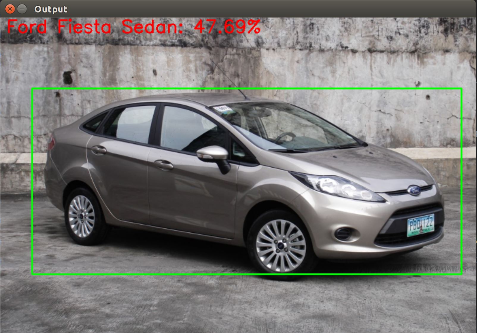
python classify.py --image samples/Ford_FiestaSedan.jpg

In which "samples/Ford_FiestaSedan.jpg" is the path to the image.

If everything is configured correctly you can see the process running:

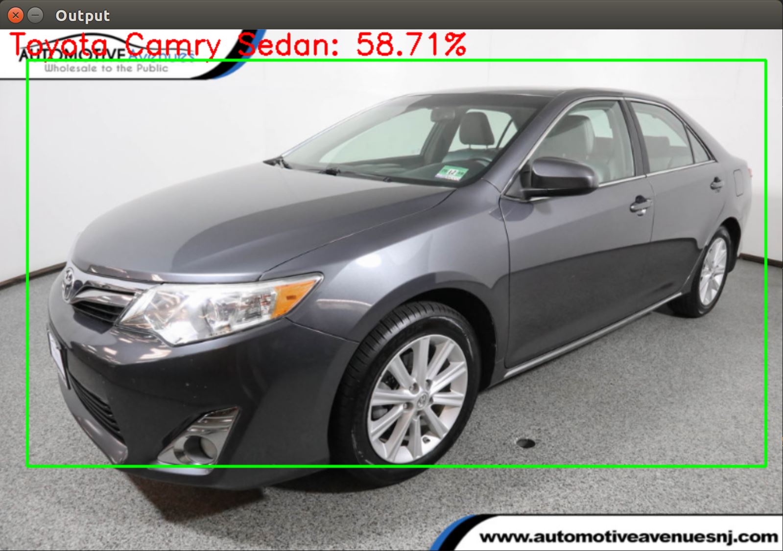
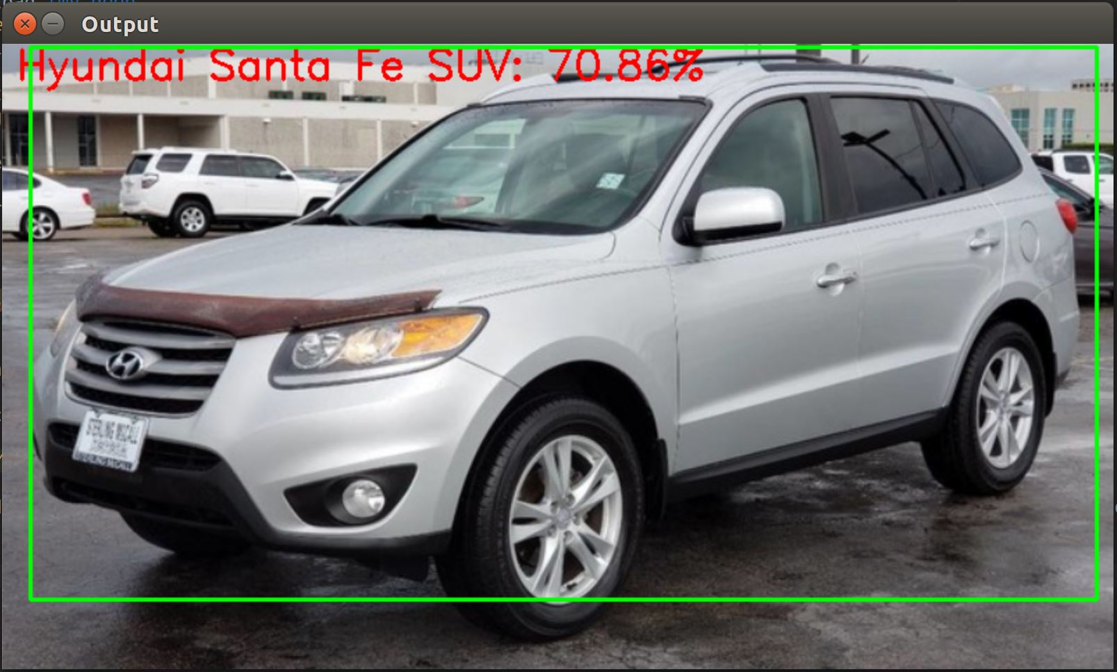
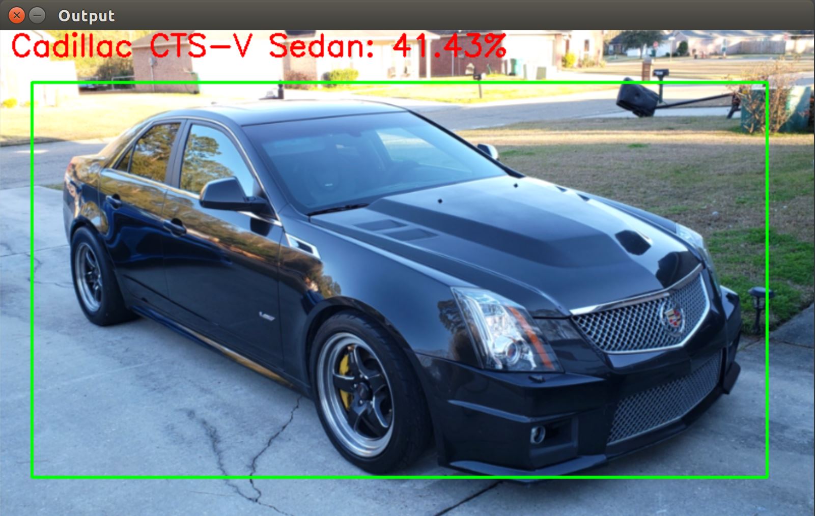
It will output the make, model and confidence score for the car in the image, for example "Ford Fiesta Sedan: 47.69%". It will also show the image with a bounding box for the car and the prediction. Here are a few examples:

Ford Fiesta	Toyota Camry Sedan

Hyundai Santa Fe SUV	Cadillac CTS-V Sedan

Training

A trained model has been provided in the link above, which is ready for classification usage. However if by any chance you would like to re-run the model training, please follow the below steps.

First you need to download the Cars dataset provided by Stanford here. After it's downloaded, put it to the root folder of this repository and unpack it by running:

tar -xvzf car_ims.tgz

It will unpack all the images to "car_ims" folder. We can now run the script which trains the model:

python myvgg_net_train.py

Please note that you will probably need a GPU to train my model. For your reference, I run my model training on Amazon Web Service with a Tesla K80 GPU (the p2.xlarge EC2 instance).

It may take a good few hours depending on your machine specification. After it completes, it will create a pickle file named myvgg_labels.pickle and four models named model_1.model, model_2.model, model_3.model and myvgg.model in the "models" folder. The first three models are created from training three fine-tuned VGGNet, and the last model is an ensemble model of the first three. I will explain the technical details of the training process later. For now you can use the myvgg.model file for classification as described in the section above.

Technical Details

Preparation

The Stanford Cars dataset is accompanied with a devkit which includes the class labels and bounding boxes for all images. These are provided in matlab format and have been converted into CSV files for easy manipulation. These CSV files are located under "annotations" folder where:

• annotations.csv contains the annotations (image path, label id, bounding box coordinates, etc.) for each image.

• class_names.csv contains all the class names.

Preprocess

A preprocess step is needed before the actual model training. This is written in the method build_data_and_labels in the file preprocess.py

In this method, the following are performed:

• Read the annotations and remove the year from the class names, so that it's left with make and model only

• Utilise the bounding box and retain the image section within the bounding box only. We will use these cropped images for training rather than the whole images as it reduces the noise and yields better performance.

• In my model training, I use VGG16 network as the base model, so each image is normalised according to VGG-specific setup such as image resize (224x224), mean subtraction, etc.

Feature Engineering

Since 2013 when the Stanford Cars dataset was first introduced, hand-crafted features for classification problems have been outperformed by deep learning models. It has been proved that deep learning models have performed consistently and extremely well such as in the ImageNet Large Scale Visual Recognition Challenge where GoogLeNet and VGGNet was the winner and runner-up respectively in 2014, and ResNet was the winner in 2015. At the moment deep learning is the de-facto state-of-the-art choice for image classification as well as many other computer vision problems.

In my project I applied the transfer learning method where I re-used an existing pre-trained deep learning network as the starting point for the task of predicting make and model of a car image. Initially I decided to pick out VGG16 and ResNet50 networks for experiments.

After some quick experiments, it appeared that the VGG16 performed better than ResNet50 for the sake of this task. Therefore I discarded the ResNet50 and continued with VGG16.

The file myvggnet/myvggnet.py contains my network model. Keras and Tensorflow are utilised for building my network. In the build method it initialises the VGG16 network without the fully connected layer. The first time you run it, the VGG16 weights is downloaded automatically if it's not downloaded before:

conv_base = VGG16(weights="imagenet", include_top=False, input_shape=config.IMAGE_DIMS)

As part of transfer learning, all the layers in VGG16 are frozen:

for layer in conv_base.layers:
    layer.trainable = False

After that a fully connected layer is added and it completes with a softmax activation:

model = Sequential()
model.add(conv_base)
        
model.add(Flatten())
model.add(Dense(1024))
model.add(Activation("relu"))
model.add(BatchNormalization())
model.add(Dropout(0.5))

model.add(Dense(classes))
model.add(Activation(finalAct))

Now the model is ready for training. The file myvgg_net_train.py is responsible for training my model. First the dataset is gone through the preprocess step as described above:

data, labels, label_binarizer = preprocess.build_data_and_labels()

The processed dataset is then split 80:20 for train and test data respectively:

(trainX, testX, trainY, testY) = train_test_split(data, labels, test_size=0.2, random_state=config.RANDOM_SEED)

ImageDataGenerator is used to generate more data for the training:

aug = ImageDataGenerator(rotation_range=25, width_shift_range=0.1,
	height_shift_range=0.1, shear_range=0.2, zoom_range=0.2,
	horizontal_flip=True, fill_mode="nearest")

Initially I fine-tuned the hyper-parameters (optimizer, number of epochs, learning rate, etc.) for one model only and achieved a decent result (precision and recall were around 0.72 on the test data). However as pointed out by various papers such as this and this, ensemble methods can often perform better than a single model. Ensemble is a technique that combines several models to produce a new model which is presumably better than individual ones. There are various methods for ensemble such as unweighted average, weighted average, majority voting, stacking, etc. For the sake of simplicity, in this project I created three models with the same structure but each uses a different optimizer (Adam, RMSprop and Adagrad). After that an ensemble model is created using unweighted averaging. The code for ensemble is provided in the method ensemble_models in the file myvggnet/myvggnet.py:

def ensemble_models(models, model_input):
    # collect outputs of models in a list
    y_models = [model(model_input) for model in models]
    # averaging outputs
    y_avg = layers.average(y_models)
    # build model from same input and avg output
    model_ens = Model(inputs=model_input, outputs=y_avg, name='ensemble')

    return model_ens

Evaluation

Under the "reports" folder there are report_1.txt, report_2.txt and report_3.txt which are the classification reports on the test data for model_1 (using Adam optimizer), model_2 (using RMSprop optimizer) and model_3 (using Adagrad optimizer) respectively. The average precision, recall, and f1-score for each single model can be seen in the tables below:

model_1 (using Adam optimizer):

	Precision	Recall	f1-score	support
micro avg	0.72	0.72	0.72	3237
macro avg	0.75	0.72	0.72	3237
weighted avg	0.76	0.72	0.72	3237

model_2 (using RMSprop optimizer):

	Precision	Recall	f1-score	support
micro avg	0.69	0.69	0.69	3237
macro avg	0.74	0.69	0.69	3237
weighted avg	0.74	0.69	0.69	3237

model_3 (using Adagrad optimizer):

	Precision	Recall	f1-score	support
micro avg	0.74	0.74	0.74	3237
macro avg	0.76	0.74	0.74	3237
weighted avg	0.77	0.74	0.74	3237

There is also an ens_report.txt which is the classification report for the ensemble model:

ensemble model:

	Precision	Recall	f1-score	support
micro avg	0.77	0.77	0.77	3237
macro avg	0.79	0.77	0.77	3237
weighted avg	0.79	0.77	0.77	3237

It's clear that the ensemble model performs better than the individual ones.

Classifying and the YOLO network

One extra point of my solution that is worth noting here is the use of YOLO network from Darknet for the task of car detection.

As described in the preprocess section, the images used for training are taken from the bounding boxes of the original images, i.e. the precise areas that contains the cars only. So in my classify.py file where the classification is actually performed, before an image input is fed through the network for prediction, the bounding box for the car in the image is extracted:

# get the car bounding box
(x, y, width, height) = detect_bounding_box(image)
# extract the area which contains the car
image = image[y:y + height, x:x + width]

The task of car detection is implemented in the method detect_bounding_box in the file car_detect.py thanks to the use of YOLO network.

Room for Improvement

• As with many other deep learning models, the more data the better. The dataset provided by Stanford has 16,185 images for 196 make and model classes. This is considered "small" data in the world of deep learning. Moreover there are imbalances where some classes are overrepresented (e.g. Audi and BMW) while others (e.g. Tesla) have only a few dozens. Hence one way to improve the performance of the system is to feed more data to the neural networks. This will definitely increase the accuracy of the prediction. Within the time constraint of this challenge, I did not have enough time to collect more data, but this is a key point for future enhancement.

• In my project I combined three deep learning models into an ensemble, and each model was run with 10 epochs. This could be improved by having more deep learning models (5 to 10 models) for the ensemble and more epochs for each model. Again this was not done due to time and resources constraint.

• Experiments with more networks. During the course of this project, I experimented with only 2 deep learning networks: VGG16 and ResNet50. There are several other networks such as AlexNet, GoogLeNet, etc. which I did not have time to try. Better performance may be yielded by exploring other networks.