Interfacing with experimental results file from TAM Air calorimeters made easy.

After collecting multiple experimental results files from a TAM Air calorimeter you will be left with multiple .xls-files obtained as exports from the device control software. To achieve a side by side comparison of theses results and some basic extraction of relevant parameters, TAInstCalorimetry is here to get this done smoothly.

Note: TAInstCalorimetry has been developed without involvement of TA Instruments and is thus independent from the company and its software.

Info / Downloads

Table of Contents

• Example Usage
  
  • Basic plotting
    
  • Getting cumulated heat values
    
  • Identifying peaks
    
  • Identifying peak onsets
    
  • Plotting by Category
    
• Installation
  
• Contributing

Example Usage

Import the tacalorimetry module from TAInstCalorimetry.

# import
import os
from TAInstCalorimetry import tacalorimetry

Next, we define where the exported files are stored. With this information at hand, a Measurement is initialized. Experimental raw data and the metadata passed in the course of the measurement are retrieved by the methods get_data() and get_information(), respectively.

# define data path
# "mycalodata" is the subfoldername where the calorimetry
# data files (both .csv or .xlsx) are stored

pathname = os.path.dirname(os.path.realpath(__file__))
path_to_data = pathname + os.sep + "mycalodata"

# Example: if projectfile is at "C:\Users\myname\myproject\myproject.py", then "mydata"
# refers to "C:\Users\myname\myproject\mycalodata" where the data is stored

# load experiments via class, i.e. instantiate tacalorimetry object with data
tam = tacalorimetry.Measurement(folder=path_to_data)

# get sample and information
data = tam.get_data()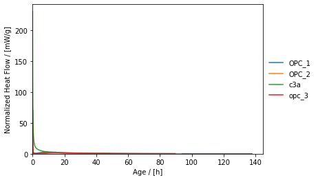
info = tam.get_information()

Basic plotting

Furthermore, the Measurement features a plot()-method for readily visualizing the collected results.

# make plot
tam.plot()
# show plot
tacalorimetry.plt.show()

Without further options specified, the plot()-method yields the following.

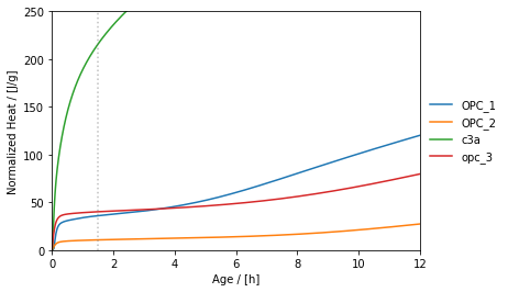
The plot()-method can also be tuned to show the temporal course of normalized heat. On the one hand, this "tuning" refers to the specification of further keyword arguments such as t_unit and y. On the other hand, the plot()-method returns an object of type matplotlib.axes._subplots.AxesSubplot, which can be used to further customize the plot. In the following, a guide-to-the-eye line is introduced next to adjuting the axes limts, which is not provided for via the plot()-method's signature.

# show cumulated heat plot
ax = tam.plot(
    t_unit="h",
    y='normalized_heat',
    y_unit_milli=False
)

# define target time
target_h = 1.5

# guide to the eye line
ax.axvline(target_h, color="gray", alpha=0.5, linestyle=":")

# set upper limits
ax.set_ylim(top=250)
ax.set_xlim(right=6)
# show plot
tacalorimetry.plt.show()

The following plot is obtained:

Getting cumulated heat values

The cumulated heat after a certain period of time target_h from starting the measurement is a relevant quantity for answering different types of questions. For this purpose, the method get_cumulated_heat_at_hours returns an overview of this parameter for all the samples in the specified folder.

# get table of cumulated heat at certain age
cumulated_heats = tam.get_cumulated_heat_at_hours(
          target_h=target_h,
          cutoff_min=10
          )
          
# show result
print(cumulated_heats)

The return value of the method, cumulated_heats is a pd.DataFrame.

Identifying peaks

Next to cumulated heat values detected after a certain time frame from starting the reaction, peaks characteristics can be obtained from the experimental data via the get_peaks-method.

# get peaks
peaks = tam.get_peaks(
    show_plot=True,
    prominence=0.00001,  # "sensitivity of peak picking"
    cutoff_min=60,  # how much to discard at the beginning of the measurement
    plt_right_s=4e5,
    plt_top=1e-2,
    regex=".*_\d"  # filter samples
    )

Tweaking some of the available keyword arguments, the following plot is obtained:

Please keep in mind, that in particular for samples of ordinary Portland cement (OPC) a clear and unambiguous identification/assigment of peaks remains a challenging task which cannot be achieved in each and every case by TAInstCalorimetry. It is left to the user draw meaningful scientific conclusions from the characteristics derived from this method.

Identifying peak onsets

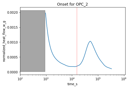
Similarly, the peak onset characteristics are accessible via the get_peak_onsets-method. The resulting plot is shown below.

# get onsets
onsets = tam.get_peak_onsets(
    gradient_threshold=0.000001,
    rolling=10,
    exclude_discarded_time=True,
    show_plot=True,
    regex="OPC"
)

Plotting by Category

For introducing the idea of plotting calorimetry data "by category" another set of experimental data will be introduced. Next to the calorimetry data alone, information on investigated samples is supplied via an additional source file. In the present example via the file mini_metadata.csv.

To begin with, a TAInstCalorimetry.tacalorimetry.Measurement-object is initialized for selected files from the specified ````path```.

import pathlib
from TAInstCalorimetry import tacalorimetry

# path to experimental calorimetry files
path = pathlib.Path().cwd().parent / "TAInstCalorimetry" / "DATA"

# initialize TAInstCalorimetry.tacalorimetry.Measurement object
tam_II = tacalorimetry.Measurement(
    path, regex="myexp.*", show_info=True, cold_start=True, auto_clean=False
)

Next, we need to connect the previously defined object to our metadata provided by the mini_metadata.csv-file. To establish this mapping between experimental results and metadata, the file location, i.e. path, and the column name containing the exact(!) names of the calorimetry files needs to be passed to the add_metadata_source-method. In our case, we declare the column experiment_nr for this purpose

# add metadata
tam.add_metadata_source("mini_metadata.csv", "experiment_nr")

Finally, a plotting by category can be carried out by one or multiple categories as shown in the following.

# define action by one category
categorize_by = "cement_name"  # 'date', 'cement_amount_g', 'water_amount_g'

# # define action by two or more categories
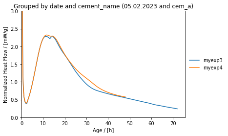
categorize_by = ["date", "cement_name"]

# loop through plots via generator
for this_plot in tam.plot_by_category(categorize_by):
    # extract parts obtained from generator
    category_value, ax = this_plot
    # fine tuning of plot/cosmetics
    ax.set_ylim(0, 3)
    # show plot
    tacalorimetry.plt.show()

This yields plots of the following kind.

Installation

Use the package manager pip to install TAInstCalorimetry.

pip install TAInstCalorimetry

Contributing

Pull requests are welcome. For major changes, please open an issue first to discuss what you would like to change.

Please make sure to update tests as appropriate.

List of contributors:

• mj-hofmann
• tgaedt

License

GNU GPLv3

Test

Code Styling