Grimon

Graphical interface to visualize multi-omics networks.

Overview

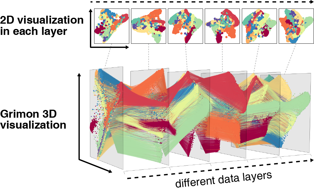
Grimon (Graphical interface to visualize multi-omics networks) visualizes high-dimensional multi-layered data sets in three-dimensional parallel coordinates. It enables users to intuitively and interactively explore their data, helping their understanding of multiple inter-layer connections embedded in high-dimensional complex data.

Installation

To install Grimon, please type the following code in your R console.

if (!require("devtools")) {
  install.packages("devtools")
}
devtools::install_github("mkanai/grimon")

Requirements

• rgl package. Grimon fully utilizes rgl's functionality to plot 3D interactive graphics using OpenGL.

Example usage

library(grimon)
# "example" and "example_col" will be loaded.
data("grimon.example")

# grimon plot function
grimon(x = example, col = example_col, label = 1:6,
       optimize_coordinates = TRUE, maxiter = 1e3,
       score_function = "angle",
       segment_alpha = 0.5)

This will plot an example figure of the above Grimon visualization in an interactive 3D window of the rgl device. You can interact with the plot using your mouse. By default, the left mouse button is used to rotate the plot (by dragging; i.e., click, hold, and move). The right mouse button is used to resize the plot, and the middle button is to change the perspective in the point of view.

Here, each argument of the grimon function corresponds to:

• x: an input matrix. The i- and i+1-th columns correspond to x- and y- values of the i-th layer.
• col: colors of points. They are also used for colors of segments (edges) unless segment_col is specified.
• label: labels of planes (layers).
• optimize_coordinates: a logical value indicating whether to optimize points coordinates across layers.
• maxiter: a maximum number of iterations for optimization by simulated annealing.
• score_function: an objective score function to minimize. Currently, it could be either "angle" or "length". If "angle", the sum of angles of segments (edges) from the flat ground (the horizontal line) will be minimized. If "length", the sum of length of segments will be minimized.
• segment_alpha: alpha transparency of segments (edges)

For a full explanation of all the arguments available, please refer to ?grimon.

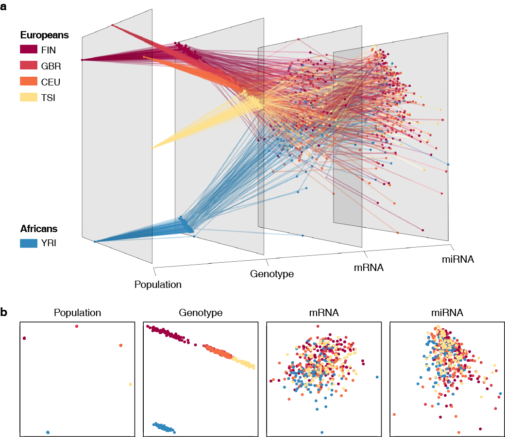
In addition to "grimon.example" (a simulated data based on the MNIST data set), we also provide additional example data constructed from publicly available multi-omics data sets: "grimon.geuvadis" (Lappalainen, T., et al., Nature, 2013) and "grimon.jointLCL" (Li, YI., et al., Science, 2016).

For each example data set, you can plot Grimon visualization via the following code. Please note that these data("grimon.XXX") commands will load the two variables into your environment, the input data, XXX (e.g. geuvadis), and the colors of points, XXX_col (e.g. geuvadis_col). Unlike "grimon.example", "grimon.geuvadis" and "grimon.jointLCL" provide the input data as a list, which exemplifies an input list explained below.

# Geuvadis Project data (Lappalainen, T., et al., Nature, 2013)
# "geuvadis" and "geuvadis_col" will be loaded.
data("grimon.geuvadis")
grimon(x = geuvadis, col = geuvadis_col,
       optimize_coordinates = TRUE, maxiter = 1e3,
       score_function = "angle",
       segment_alpha = 0.5)

# JointLCL data (Li, YI., et al., Science, 2016)
# "jointLCL" and "jointLCL_col" will be loaded.
data("grimon.jointLCL")
grimon(x = jointLCL, col = jointLCL_col,
       optimize_coordinates = TRUE, maxiter = 1e3,
       score_function = "angle",
       segment_alpha = 0.5)

Prepare your input

Grimon accepts an input matrix, data.frame, or list. If matrix or data.frame is supplied, basically it should be n x 2m matrix, where n represents a number of points (samples) and m represents a number of planes (layers). If list is supplied, Grimon automatically combines all the elements in the same order of the original list.

For example, assume you have multiple original data matrix in a list format, and want to plot Grimon visualization of the first two PCs across different data sets. You could generate your input to Grimon using the following code.

original_data = list(A = ...,
                     B = ...,
                     C = ..., ...)

# list
input_list = lapply(original_data, function(mat) {
  # returns the first two PCs
  prcomp(mat, scale=T)$x[,1:2]
})

# matrix
input_mat = do.call(cbind, input_list)

If the number of samples is different across multiple data sets (layers), you could set missing observations for a specific layer as NA. Missing points are not connected by edges. One easy approach to do this (under this example situation) is shown below.

input_mat = matrix(nrow = length(all_samples), ncol = 2,
                   dimnames = list(all_samples, c("PC1", "PC2")))
. = lapply(original_data, function(mat) {
  input_mat[samples_A] = prcomp(mat, scale=T)$x[,1:2]
})

Save figures

To save your figure, please use rgl.snapshot or rgl.postscript. While rgl.postscript saves your figure in a vector graphics, it doesn't support alpha transparency and the resulting file becomes too large when the figure contains too many points and edges. On the other hand, one of the limitations of rgl.snapshot is that users couldn't specify resolution of the image. If you want to generate a high-resolution figure for publication, we recommend you to use the option windowRect to maximize your rgl device size as wide as possible.

# E.g., this will enlarge your window size four times bigger than the default.
grimon(..., windowRect = c(0, 0, 3200, 2400))
rgl.snapshot("image.png")

# or, you can specify your window size ad-hoc.
grimon(...)
# -- some interaction --
par3d(windowRect = c(0, 0, 3200, 2400))
rgl.snapshot("image.png")

You could also plot the two-dimensional figures of each layer (as shown below) with plot_2d_panels = True option. They will be plotted in the default device, thus you could save them using a usual pdf(...) function, for example.

Example figures

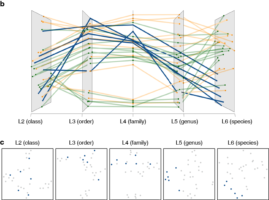
Example 1: Metagenome data (Maeda, Y., et al., Arthritis Rheumatol., 2016)

Example 2: the Geuvadis Project (Lappalainen, T., et al., Nature, 2013)

Citation

When using Grimon, please cite the following paper.

• Kanai, M., Maeda, Y. & Okada, Y. Grimon: Graphical interface to visualize multi-omics networks. Bioinformatics (2018). doi:10.1093/bioinformatics/bty488

Contact

Masahiro Kanai (mkanai@g.harvard.edu)

http://mkanai.github.io/