Feature Selection and Extraction (FSE)

This repository includes different analyses to explore gene expression data using different Machine Learning approaches:

• Principal Component Analysis (PCA)
• t-distributed Stochastic Neighbor Embedding (tSNE)
• Gaussian Mixture Model (GMM) analysis
• Decision trees

All the analyses listed above takes the same input: a data table with observations at rows and variables at columns. The input table could be provided in any of the next two formats: Excel or csv. Tables should include a header with the names of the variables. In addition, the first and second columns should have the sample class and a unique sample identifier respectively.

Apart from this repository, you might consider to have a look to Classification/ for additional further analyses.

PCA_analysis

This repository includes a MATLAB script to perform a dimensionality reduction analysis using the Principal Components method.

Principal component analysis for clustering gene expression data. Bioinformatics (2001).

Input

Data is read from a table in CSV or Excel file with the format described before.

Output

The script computes PCA using the singular value decomposition method by using function pca from MATLAB's statistichal toolbox. Next are listed the figures and output files:

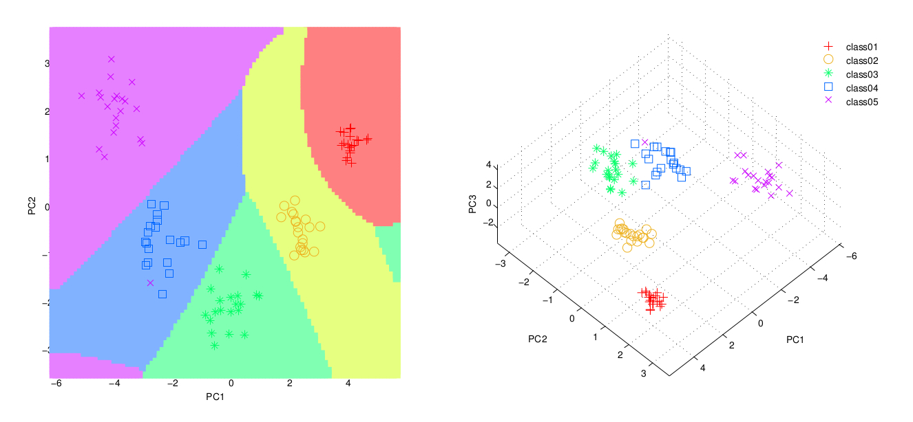
1. A scatter-plot with the two first components and the classification resulting from a Quadratic Discriminant Analysis (QDA).
2. A scatter-plot with the three first components. Before plotting them, the components are rotate using the varimax transformation to find the optimum orientation.
3. A report showing the information content of each componenent (and up to which the 95% of the variance is explained).
4. A CSV file, in the same folder of the input data with same name and prefix __PCA, with the PCA coordinates. See example here.
5. At the end of the script, the program asks if you want to identify a subset of data points in the 2D plot. We refer to this kind subset as superclass. If you click Yes, a new window will be opened with the PCA scatter-plot. Then, you can click on each single point one by one or drag over the region you are interested in. Once your selection is done, press Enter to finish and an additional text file with the names of the selected data-points will be output. It will be saved with the name of the input file, in the same folder and the prefix __PCA_superclass. An example of this output can be found here.

Further analysis

Consider the use of GMM_clustering from Classification/ to cluster the results using Gaussian Mixture Models or any of thr SVM scripts from to compute a boundary in bewtween two subpopulations. If you have selected a superclass, you might consider to use the BDT analysis.

tSNE_analysis

This repository includes a set of scripts to perform a dimensionality reduction analysis using the t-Distributed Stochastic Neighbor Embedding (tSNE) method.

Visualizing High-Dimensional Data Using t-SNE. Journal of Machine Learning Research (2008).

Dependencies

The main script, tSNE_analysis.m, depends on the MATLAB implementation of the tSNE method. The original code from the tSNE algorithm can be found in Simple_tSNE/. Before running the program check the path in SETTINGS, at the begining of the main script.

Input

Data is read from a table in CSV or Excel file with the format described before. A pick-file menu will be displayed once you run the script. Next are listed a set of parameters that you can set up:

1. PCA_level, the percentage of variace to keep for data preprocessing. The tSNE method preprocesses the input data using PCA and choosing a given number of initial dimensions to compute an initial solution. Instead of choosing an arbitrary number of components, the program performs PCA and chooses the number of components comprising a given level of variability. By default, this level is set to keep the 95% of the variance. To skip the preprocessing step, set this variable to 100%.
2. seed, the random generator's seed. tSNE is an stochastic method that will produce a different result every time. For repeatability, the randomness is controlled by fixing the seed of the random generator. By default,it set as zero. Use any other value to generate alternative solutions.

Output

The script outputs the next files and figures:

1. A scatter-plot with the 2D PCA and the classification from the Quadratic Discriminant Analysis (QDA).
2. A scatter-plot with the 3D PCA plot. Data are rotated using varimax transformation to find the optimum orientation.
3. A report showing the information content of each componenent (and up to which the given percentage of the variance is explained).
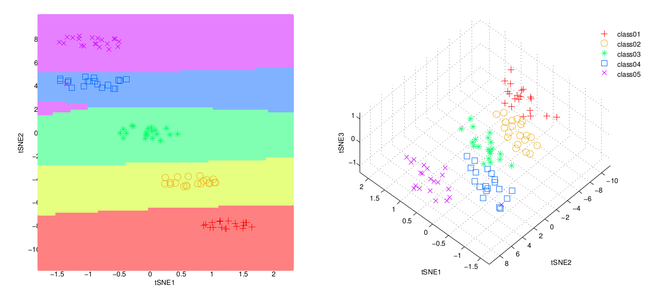
4. A scatter-plot with the 2D tSNE and the classification from the Quadratic Discriminant Analysis (QDA). Coordinates are also saved to a file in the same folder than the input file.
5. A scatter-plot with the 3D tSNE plot. Data are rotated using varimax transformation. Coordinates are also saved to a file in the same folder than the input file.
6. Before plotting the 3D tSNE, users may interact with the 2D plot to manually pick a subset of samples. We refer to this subsets as superclass. During selection, click on each single point one by one or drag over the region you are interested in. Once your selection is done, press Enter to finish. A text file with the names of the selected data-points will be output. It will be saved with the name of the input file, in the same folder and the prefix __tSNE_superclass. An example of this output can be found here.

Further analysis

Consider the use of gmm_clustering to cluster the results using Gaussian Mixture Models. You can also use any of the SVM scripts from Classification/ to compute a boundary in bwtween two subpopulations. If you have selected a superclass, you might consider to use the BDT analysis.

GMM_analysis

This repository includes a scripts to perform a Gaussian Mixture Model (GMM) analysis to decompose qPCR data into Gaussian signals.

Mixture-model based estimation of gene expression variance. Bioinformatics (2010).

Input

Data is read from a table in CSV or Excel file with the format described before. A pick-file menu will be displayed once you run the script. Next are listed a set of parameters that you can set up:

1. seed, the random generator's seed. tSNE is an stochastic method that will produce a different result every time. For repeatability, the randomness is controlled by fixing the seed of the random generator. By default,it set as zero. Use any other value to generate alternative solutions.

Output

The script fits the data to a GMM with diferent modes, from one to the total number of classes in the data, for each single gene using gmdistribution from Matlab's statistical toolbox. For each of the GMM, the Akaike's information criterion is computed and the model that minimises it is reported. Next are listed the figures and output files:

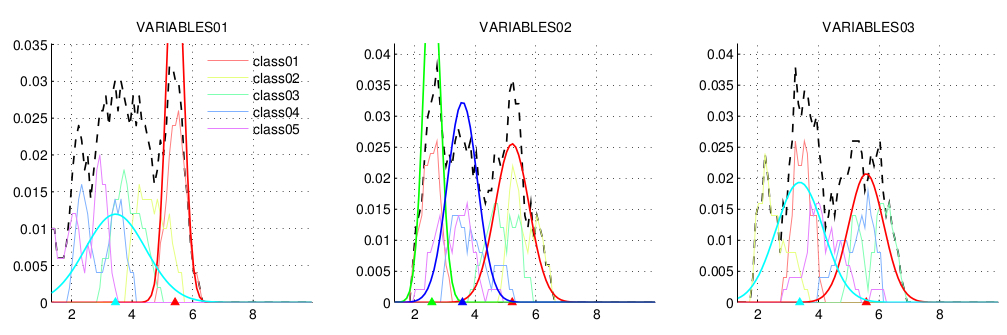
1. A figure with 3x3 subplot showing the density of the expression profiles for each single gene across all the samples (in black) and for each of the classes (in different colors). The GMM are overlap, with each of the independent modes in different colors. The mean of each Gaussian is marked in the x-axis with a triangle. Each figure is saved as a PDF in the same folder of the input file, with the same name and the prefix __qPCR. An example of this output can be found here.
2. A CSV file with the hyperparameters of the GMM for each of the genes: (i) the mean and (ii) the standard deviation (the squared root of the variance). An example of this output can be found here.

BDT_analysis

This repository performs an emsembled classificator using a Bagger Decision Tree (BDT). Note that a BDT is not a random forest.

A comparative study of different machine learning methods on microarray gene expression data. BMC Genomics (2008).

Input

Data is read from a table in CSV or Excel file with the format described before. A pick-file menu will be displayed once you run the script. Next are listed a set of parameters that you can tune:

1. NoDT, the Number of Decission Trees to train the classifier. By default is set to 100.

2. seed, the random generator's seed. For repeatability, the randomness is controlled by fixing the seed of the random generator. By default,it set as zero. Use any other value to generate alternative solutions.

Output

The script outputs a set of plots with statistics measuring the stability of the BDT and assessing the results.

1. Biased evaluation of the BDT by predicting the classes of the trainning data set.
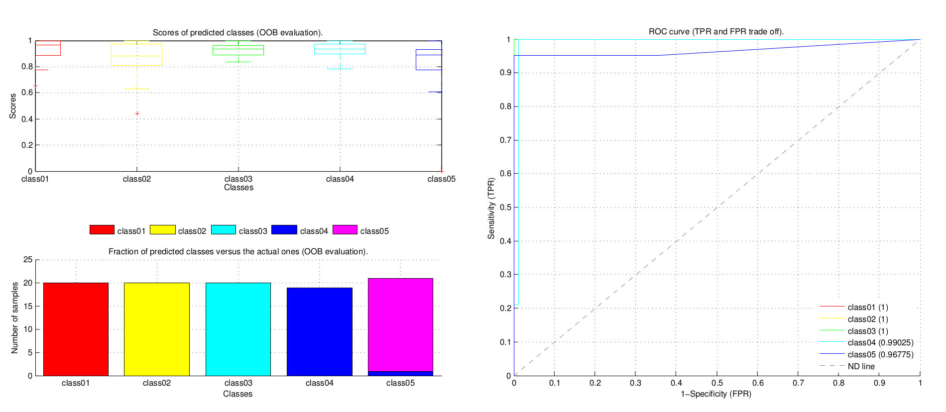
2. Fair evaluation of the BDT by predicting the out-of-bag (OOB) observations.
3. Evaluation of the stability of the BDT by computing the OOB error (missclasication probability) and the margin (the difference between the score for the actual class and the largest one for other classes) for each individual tree and the cumulative value for a given number of trees.
4. The predictor importance, that averages the changes in the risk due to split on every predictor at each node for the whole ensemble. This risk depends on the seleted split criterion (typically GDI that measure the impurity of the node).
5. The variable relevance, measured as the increase in the OOB error when the values of the variables are permutted for every tree, then averaged over the entire ensemble and lastly divided by the standard deviation.
6. ROC curve, the Receiver Operating Characteristic (ROC) curve illustrates the performance of the BDT by analysing the trade off between sensitivity and specificcity. The no-discrimination (ND) line is the theoretical behaviour when classes are randomly asingned. The higher the area under the ROC curves the better the performance.
7. Similarly to the ROC curve, the Precission Recall (PR) curve summarises the behaviour of the classifier.
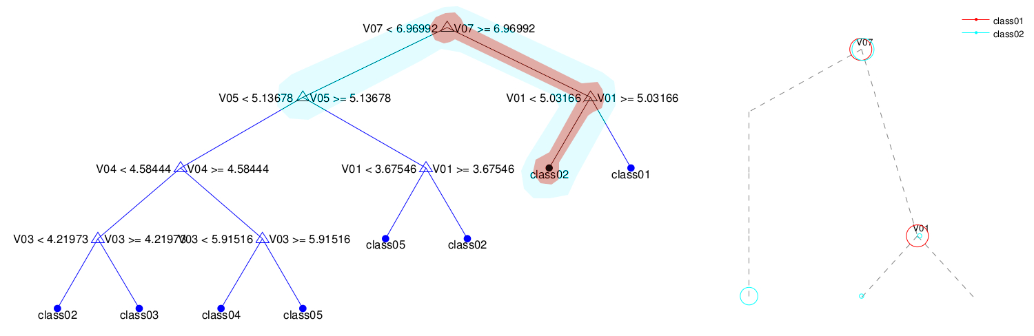
8. The BDT as a tree plot.
9. Finally, the script allows you to track a subpopulation across the BDT. We refer to this subpopulation as a super-class. To see how a superclass is partitioned along the BDT, say Yes on the dialog menu and pick a one-column text file with the identifiers of the data points you want to track. Only the leaves of the trees with any of these data points will be displayed. Each subpopulation within the superclass will be displayed as a circle of different colors. The sizes of the circles at each node are proportional to the number of samples in the superclass.