Causal discovery with the GES algorithm goes along the same lines as the PC algorithm. We again take the examle in chapter 2 of Judea Pearl's book. The causal model we are going to study can be represented using the following DAG:
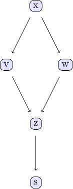
We can easily create some sample data that corresponds to the causal structure described by the DAG. For the sake of simplicity, let's create data from a simple linear model that follows the structure defined by the DAG shown above:
using CausalInference
using TikzGraphs
using Random
Random.seed!(1)

# Generate some sample data to use with the GES algorithm

N = 2000 # number of data points

# define simple linear model with added noise
x = randn(N)
v = x + randn(N)*0.25
w = x + randn(N)*0.25
z = v + w + randn(N)*0.25
s = z + randn(N)*0.25

df = (x=x, v=v, w=w, z=z, s=s)
With this data ready, we can now see to what extent we can back out the underlying causal structure from the data using the GES algorithm. Under the hood, GES uses a score to determine the causal relationships between different variables in a given data set. By default, ges uses a Gaussian BIC to score different causal models.
est_g, score = ges(df; penalty=1.0, parallel=true)In order to investigate the output of the GES algorithm, the same plotting function applies.
tp = plot_pc_graph_tikz(est_g, [String(k) for k in keys(df)])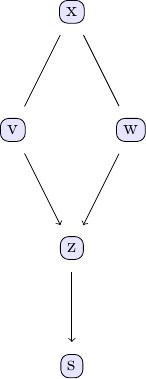
We can compare with the output of the PC algorithm
est_g2 = pcalg(df, 0.01, gausscitest)
est_g == est_g2
For the data using this seed, both agree.
Instead of GES which greedily tries to maximize the BIC score, we can also sample the posterior distribution over CPDAGs corresponding to the BIC score. We have implemented the Causal Zig-Zag for this. (See: M. Schauer, M. Wienöbst: Causal structure learning with momentum: Sampling distributions over Markov Equivalence Classes of DAGs. (https://doi.org/10.48550/arXiv.2310.05655))
iterations = 50_000
n = length(df) # vertices
κ = n - 1 # max degree
penalty = 2.0 # increase to get more edges in truth
Random.seed!(101)
C = cor(CausalInference.Tables.matrix(df))
score = GaussianScore(C, N, penalty)
gs = @time causalzigzag(n; score, κ, iterations)
gs contains the samples of the chain and weight information. The following two lines aggregate this information to obtain a posteriori probabilities of different CPDAGs.
graphs, graph_pairs, hs, τs, ws, ts = CausalInference.unzipgs(gs)
posterior = sort(keyedreduce(+, graph_pairs, ws); byvalue=true, rev=true)
posterior is a dictorarity assigning each CPDAG is (marginal) a-posteriori probability using the prior with parameter penalty. (Graphs are represented as vector of directed edges.)
  [1=>2, 1=>3, 2=>1, 2=>4, 3=>1, 3=>4, 4=>5]                                           => 0.997285
  [1=>2, 1=>3, 2=>1, 2=>3, 2=>4, 3=>1, 3=>2, 3=>4, 4=>2, 4=>3, 4=>5, 5=>4]             => 0.000590422
  [1=>2, 1=>3, 1=>5, 2=>1, 2=>4, 3=>1, 3=>4, 4=>5]                                     => 0.000565705
  [1=>2, 1=>3, 1=>4, 2=>1, 2=>4, 3=>1, 3=>4, 4=>5]                                     => 0.000543214
  [1=>2, 1=>3, 2=>1, 2=>4, 2=>5, 3=>1, 3=>4, 4=>5]                                     => 0.000517662
  ...
From this we see that the maximum a posterior graph coincides with the GES estimate and has high posterior weight, showing that the result of the GES algorithm is not incidental.
We also provide an implementation of the exact optimization algorithm by Silander and Myllymäki (2006). Given observed data, it outputs the CPDAG representing the set of DAGs with maximum BIC score. The algorithm is exact, meaning it is guaranteed that the optimal CPDAG with regard to the BIC score is found.
The time and memory complexity of the algorithm is in the order of
It can be called similar to GES:
est_g = exactscorebased(df; penalty=1.0, parallel=true)Reference:
- Silander, T., & Myllymäki, P. (2006). A simple approach for finding the globally optimal Bayesian network structure. In Uncertainty in Artificial Intelligence (pp. 445-452).