opda: optimal design analysis

Docs | Source | Issues | Changelog

Design and analyze optimal deep learning models.

Optimal design analysis (OPDA) combines an empirical theory of deep learning with statistical analyses to answer questions such as:

1. Does a change actually improve performance when you account for hyperparameter tuning?
2. What aspects of the data or existing hyperparameters does a new hyperparameter interact with?
3. What is the best possible score a model can achieve with perfectly tuned hyperparameters?

This toolkit provides everything you need to get started with optimal design analysis. Jump to the section most relevant to you:

• Installation
• Quickstart
• Resources
• Citation
• Contact

Installation

Install opda via pip:

$ pip install opda

See the Setup documentation for information on optional dependencies and development setups.

Quickstart

Let's evaluate a model while accounting for hyperparameter tuning effort.

A key concept for opda is the tuning curve. Given a model and hyperparameter search space, its tuning curve plots model performance as a function of the number of rounds of random search. Thus, tuning curves capture the cost-benefit trade-off offered by tuning the model's hyperparameters.

We can compute tuning curves using the opda.nonparametric.EmpiricalDistribution class. Beforehand, run several rounds of random search, then instantiate EmpiricalDistribution with the results:

>>> from opda.nonparametric import EmpiricalDistribution
>>>
>>> ys = [  # accuracy results from random search
...   0.8420, 0.9292, 0.8172, 0.8264, 0.8851, 0.8765, 0.8824, 0.9221,
...   0.9456, 0.7533, 0.8141, 0.9061, 0.8986, 0.8287, 0.8645, 0.8495,
...   0.8134, 0.8456, 0.9034, 0.7861, 0.8336, 0.9036, 0.7796, 0.9449,
...   0.8216, 0.7520, 0.9089, 0.7890, 0.9198, 0.9428, 0.8140, 0.7734,
... ]
>>> dist_lo, dist_pt, dist_hi = EmpiricalDistribution.confidence_bands(
...   ys=ys,            # accuracy results from random search
...   confidence=0.80,  # confidence level
...   a=0.,             # (optional) lower bound on accuracy
...   b=1.,             # (optional) upper bound on accuracy
... )

Beyond point estimates, opda offers powerful, nonparametric confidence bands. The code above yields 80% confidence bands for the probability distribution. You can use the estimate, dist_pt, to evaluate points along the tuning curve:

>>> n_search_iterations = [1, 2, 3, 4, 5]
>>> dist_pt.quantile_tuning_curve(n_search_iterations)
array([0.8456, 0.9034, 0.9089, 0.9198, 0.9221])

Or, better still, you can plot the entire tuning curve with confidence bands, and compare it to a baseline:

>>> from matplotlib import pyplot as plt
>>> import numpy as np
>>>
>>> ys_old = [  # random search results from the baseline
...   0.7440, 0.7710, 0.8774, 0.8924, 0.8074, 0.7173, 0.7890, 0.7449,
...   0.8278, 0.7951, 0.7216, 0.8069, 0.7849, 0.8332, 0.7702, 0.7364,
...   0.7306, 0.8272, 0.8555, 0.8801, 0.8046, 0.7496, 0.7950, 0.7012,
...   0.7097, 0.7017, 0.8720, 0.7758, 0.7038, 0.8567, 0.7086, 0.7487,
... ]
>>> ys_new = [  # random search results from the new model
...   0.8420, 0.9292, 0.8172, 0.8264, 0.8851, 0.8765, 0.8824, 0.9221,
...   0.9456, 0.7533, 0.8141, 0.9061, 0.8986, 0.8287, 0.8645, 0.8495,
...   0.8134, 0.8456, 0.9034, 0.7861, 0.8336, 0.9036, 0.7796, 0.9449,
...   0.8216, 0.7520, 0.9089, 0.7890, 0.9198, 0.9428, 0.8140, 0.7734,
... ]
>>>
>>> ns = np.linspace(1, 5, num=1_000)
>>> for name, ys in [("baseline", ys_old), ("model", ys_new)]:
...   dist_lo, dist_pt, dist_hi = EmpiricalDistribution.confidence_bands(
...     ys=ys,            # accuracy results from random search
...     confidence=0.80,  # confidence level
...     a=0.,             # (optional) lower bound on accuracy
...     b=1.,             # (optional) upper bound on accuracy
...   )
...   plt.plot(ns, dist_pt.quantile_tuning_curve(ns), label=name)
...   plt.fill_between(
...     ns,
...     dist_hi.quantile_tuning_curve(ns),
...     dist_lo.quantile_tuning_curve(ns),
...     alpha=0.275,
...     label="80% confidence",
...   )
[...
>>> plt.xlabel("search iterations")
Text(...)
>>> plt.ylabel("accuracy")
Text(...)
>>> plt.legend(loc="lower right")
<matplotlib.legend.Legend object at ...>
>>> # plt.show() or plt.savefig(...)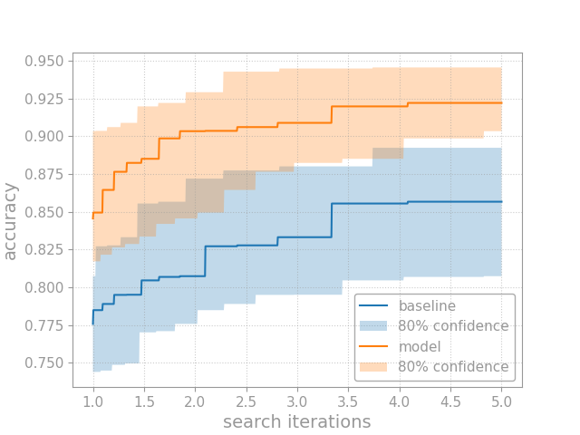

See the Usage, Examples, or Reference documentation for a deeper dive into opda.

Resources

For more information on OPDA, checkout our paper: Show Your Work with Confidence: Confidence Bands for Tuning Curves.

Citation

If you use the code, data, or other work presented in this repository, please cite:

@misc{lourie2023work,
    title={Show Your Work with Confidence: Confidence Bands for Tuning Curves},
    author={Nicholas Lourie and Kyunghyun Cho and He He},
    year={2023},
    eprint={2311.09480},
    archivePrefix={arXiv},
    primaryClass={cs.CL}
}

Contact

For more information, see the code repository, opda. Questions and comments may be addressed to Nicholas Lourie.