multiple_incidence
baptiste Auguié -- 22 June, 2014
The other demos present calculations either at a fixed incidence angle along z, typically (but not necessarily) a symmetry axis of the cluster, or with full angular averaging. This demo features the intermediate situation, where a fixed cluster is studied with multiple angles of incidence. Typical applications would be dispersion plots with linear polarisation, but it is also interesting to observe the angular dependence of optical activity.
# dielectric function
wvl <- seq(400, 900)
gold <- epsAu(wvl)

# two clusters
cl <- cluster_chain(N=2, pitch=100)

cl2 <- cluster_helix(5, R0=200, pitch=150,
                          delta=pi/2, delta0=0, right=TRUE,
                          a=50, b=50/2, c=50/2,
                          angles="helix")
hel <- helix(N = 5, R0 = 200, pitch = 150, delta = pi/2,
             delta0 = 0, right = TRUE)

# visualise
lines3d(hel$smooth, lwd=1, col="red")
  shift <- cbind(rep(1000, nrow(cl$r)),0,0)
rgl.ellipsoids(cl$r+cbind(rep(-500, 2),0,0), cl$sizes, cl$angles, col="gold")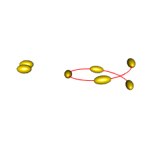
solving CD equations for two polarisations and a range of angles with rotations along x, y, z (uncoupled).
Angles <- rep(seq(0, pi/2, length=12), 3)
Axes <- rep(c('x','y','z'), each=12)

results <- dispersion_spectrum(cl, gold, angles=Angles, axes = Axes,
                               polarisation="linear")

test <- melt(results, meas="value")

ggplot(subset(test, type == "extinction"),
       aes(wavelength, value, colour=angles, group=angles)) +
  facet_grid(axes ~ polarisation, scales="free") +
  geom_line() +
  labs(y=expression(sigma[ext]*" /"*nm^2),
       x=expression(wavelength*" /"*nm), colour="incident angle")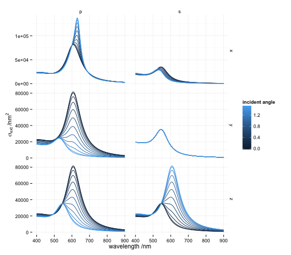
variables <- expand.grid(Angles = seq(0, 2*pi, length=36),
Axes = c('x','y','z'))
results <- dispersion_spectrum(cl2, gold, angles=variables$Angles, axes = variables$Axes,
polarisation="circular")
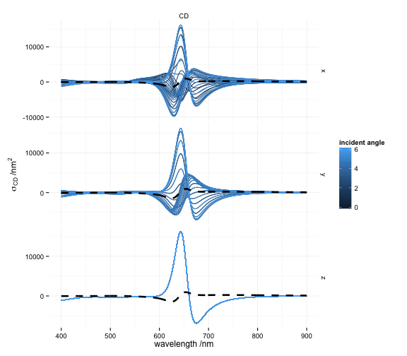
average <- circular_dichroism_spectrum(cl2, material = gold)
ggplot(subset(results, polarisation == "CD"), aes(wavelength, value)) +
facet_grid(axes ~ polarisation, scales="free") +
geom_line(aes(colour=angles, group=angles)) +
geom_line(data=subset(average, type == "CD" & variable =="extinction"), linetype=2, size=1.2) +
labs(y=expression(sigma[CD]*" /"*nm^2),
x=expression(wavelength*" /"*nm), colour="incident angle")