Integrator performs much better with a recurrent transform of 1.12 - 1.15

[arvoelke]

I did a little benchmarking of an integrator network, for several different inputs:

• Cosine
• Step-function
• Zero (holding steady at 1)

I measured the RMSE across multiple trials with different seeds, while varying the gain on the recurrent feedback.

For the reference simulator, a recurrent transform of 1 is optimal. But here, I'm getting 1.12 - 1.15, depending on the kind of input. I'm not using any interneurons, and I'm using a fairly long time-constant (100 ms).

Might be useful to eventually have a collection of similar benchmarks in a regression test framework.

from collections import defaultdict

import numpy as np
from pandas import DataFrame

import matplotlib.pyplot as plt
import seaborn as sns

import nengo_loihi; nengo_loihi.set_defaults()
import nengo
from nengo.utils.numpy import rmse
from nengolib.signal import s

n_neurons = 300
conn_tau = 0.1
probe_tau = 0.005
dt = 0.001
sim_t = 2*np.pi
simulator = nengo_loihi

data = defaultdict(list)
for desc, output in [('Cosine', np.cos),
                     ('Step', 1. / sim_t),
                     ('Zero', lambda t: 1 if t <= 1 else 0)]:
    for seed in range(5):
        for transform in np.linspace(1.05, 1.2, 10):
            print("desc=%s, seed=%d, transform=%s" % (desc, seed, transform))

            with nengo.Network() as model:
                u = nengo.Node(output=output)
                x = nengo.Ensemble(n_neurons, 1, seed=seed)

                nengo.Connection(u, x, synapse=conn_tau, transform=conn_tau)
                nengo.Connection(x, x, synapse=conn_tau, transform=transform,
                                 solver=nengo.solvers.LstsqL2(weights=True))

                p_x = nengo.Probe(x, synapse=probe_tau)
                p_ideal = nengo.Probe(u, synapse=~s * nengo.Lowpass(probe_tau))

            builder_model = simulator.builder.Model(dt=dt)
            # builder_model.inter_tau = inter_tau
            # assert builder_model.inter_n == 10  # sanity check
            # builder_model.inter_n = inter_n
            # builder_model.inter_noise_exp = 5
            with simulator.Simulator(network=model, model=builder_model, dt=dt) as sim:
                sim.run(sim_t)

            data['x'].append(sim.data[p_x].squeeze())
            data['Input'].append(desc)
            data['RMSE'].append(rmse(sim.data[p_x], sim.data[p_ideal]))
            data['Seed'].append(seed)
            data['Transform'].append(transform)

df = DataFrame(data)
plt.figure()
plt.title("Integration Performance")
sns.lineplot(data=df, x="Transform", y="RMSE", hue="Input", ci=95)
plt.show()

Also see #90 which may be related.

[tcstewar]

Very useful..... I'd be curious to look at whether this is mostly due to the U/V overflow, or due to the V being reset to zero, or due to some other problem....

[tbekolay]

I don't think it's due to a bug per se, I think Loihi tuning curves are consistently lower than the tuning curves we're used to in Nengo, which we try to account for in decoder solving, but regardless at a given x a neuron is only ever going to fire at the rate you would expect in Nengo, or lower than that rate due to the discretization. Given that, it's not too surprising that upping the strength on the connection would help. I think any kind of overflow would give a much worse RMSE, but that's just a guess.

[arvoelke]

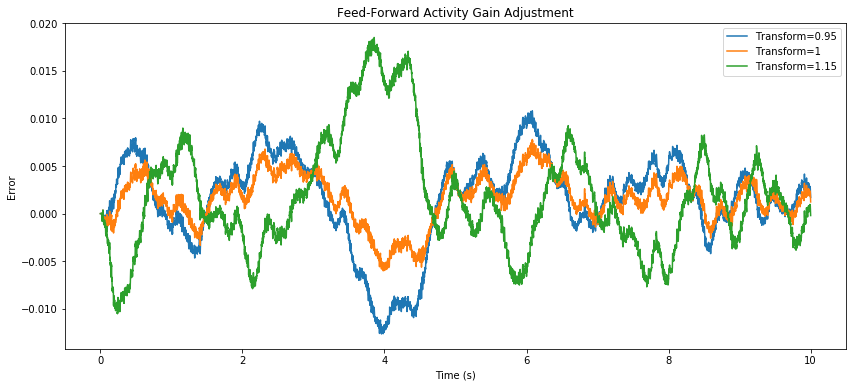
What are some of the challenges when it comes to using the quantized version of their neuron model to estimate the tuning curves? I haven't looked at this part of the code, but thinking purely about the emulator, could we do something like nengolib.solvers.Temporal to get better decoders, or derive some steady-state equations that somehow take quantization into account?

However, these questions might not tap into what's going on here, as I'm seeing, in the feed-forward case, that an output transform of 1 is better than 1.15. Note that, by linearity, applying a transform to the probed value is equivalent to rescaling the decoders, which in turn is equivalent to rescaling the y-axis on the tuning curves. And what we're seeing here is that the transform that makes things best for the recurrent case actually makes things worse for the feed-forward case.

(Note: y-axis is error.) From this, I'm thinking that a tuning shift from quantization error is not the main problem. It seems as though there's something more subtle going on pertaining to the dynamics of the system. This is not to rule out quantization effects as entirely irrelevant, however, as they could still play some important role in the context of a recurrent feedback loop.

import numpy as np
import matplotlib.pyplot as plt

import nengo
import nengo_loihi; nengo_loihi.set_defaults()
from nengolib import DoubleExp

sim_t = 10
freq = 5
rms = 0.3
tau_conn = 0.1
tau_probe = 1.0

with nengo.Network() as model:
    u = nengo.Node(nengo.processes.WhiteSignal(period=sim_t, high=freq, rms=rms, y0=0))
    
    x = nengo.Ensemble(100, 1)
    
    nengo.Connection(u, x, synapse=tau_conn)
    
    p_x = nengo.Probe(x, synapse=tau_probe)
    p_u = nengo.Probe(u, synapse=DoubleExp(tau_conn, tau_probe))
    
with nengo_loihi.Simulator(model) as sim:
    sim.run(sim_t)

plt.figure(figsize=(14, 6))
plt.title("Feed-Forward Activity Gain Adjustment")
for transform in (0.95, 1, 1.15):
    plt.plot(sim.trange(), transform*sim.data[p_x] - sim.data[p_u],
             label="Transform=%s" % transform)
plt.legend()
plt.xlabel("Time (s)")
plt.ylabel("Error")
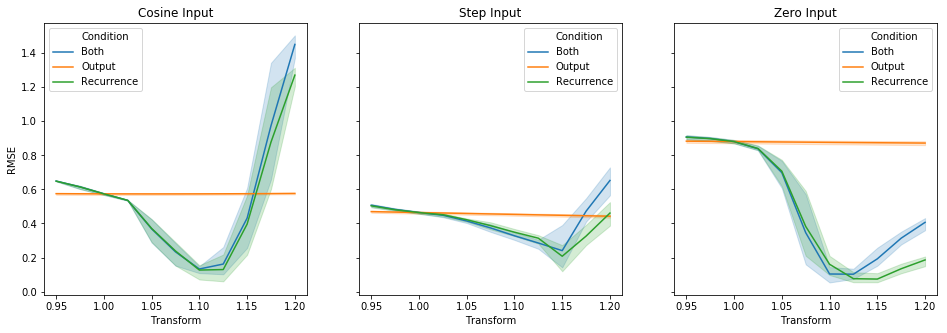
plt.show()

To get a better understanding of what could be going on here, I re-ran the initial experiment at the top, in three different conditions: (1) varying only the output gain, similar to the above feed-forward experiment, (2) varying only the recurrent gain (as done in the original post), and (3) varying both gains together -- while keeping everything else fixed. Each subplot corresponds to a different input type, and each line is a separate condition.

full_data = defaultdict(list)
for label, data in (('Both', data_both), ('Output', data_output), ('Recurrence', data_rec)):
    for name, column in data.items():
        full_data[name].extend(column)
    full_data['Condition'].extend([label] * len(column))
df = DataFrame(full_data)
fig, ax = plt.subplots(1, 3, figsize=(16, 5), sharey=True)
for i, desc in enumerate(('Cosine', 'Step', 'Zero')):
    ax[i].set_title("%s Input" % desc)
    sns.lineplot(data=df[df['Input'] == desc], ax=ax[i],
                 x="Transform", y="RMSE", hue="Condition", ci=95)
fig.show()

Adjusting only the recurrence seems slightly better than adjusting both in some cases, although the 95% confidence intervals overlap at the optimal values. This makes sense when you look at the feed-forward results, since the difference in error there is relatively quite small.

Taken together with the feed-forward observation, this appears to me to be consistent with there being dynamics other than Lowpass(tau) dominating the feedback connection. The next step that I see, after I look more at the code, is to probe the PSC of each neuron within the emulator -- to verify that it is a first-order lowpass with the prescribed tau. Is this probing possible? A different tau wouldn't explain this, unless different synapses could have different values of tau. I expect something more complicated to be going on... Depending on how this pans out, I would want to look into what Terry is saying about U/V overflow, to see what's going on there. Feel free to assign this issue to me.

[tcstewar]

The next step that I see, after I look more at the code, is to probe the PSC of each neuron within the emulator -- to verify that it is a first-order lowpass with the prescribed tau. Is this probing possible?

That sounds like an excellent idea. I don't think we have a built-in way of probing the PSC at the moment, but it's definitely available from the chip. At the moment we probe the V value, and what you want is the U value, which is accessible in the same way.

[hunse]

I don't think we have a built-in way of probing the PSC at the moment, but it's definitely available from the chip.

Conveniently, I added this in 4bec822 yesterday for my own purposes. You can probably cherry-pick it to your own branch if you want to play around with probing input currents.

[hunse]

I've done some exploring. I think this behaviour is related to a number of factors in the overall discretization done by the chip, but I've found one major factor, and the good news is I think I can fix it.

In CxGroup.discretize (where all the action happens in turns of turning the real-valued model into a fixed-point one), I compute two factors: u_infactor and v_infactor. These represent how much we have to scale u and v down by to compensate for the fact that as they have smaller decays, it takes longer for their values to go to zero, and thus each spike has a bigger effect.

I was computing these values based on the ideal math, which is what would happen if we had real values multiplied by 1 - decay every timestep. However, because the decay is happening in integer values, there's rounding down that happens. (For example, if you start with 7 and decay it by a value of 0.5, you get 3. Decay that again and you get 1. This is quite different from the ideal series of 7, 3.5, 1.75.)

Taking this rounding into account when computing u/v infactors seems to help integrator performance considerably. Now I just have to figure out an efficient way to compute these new values, as well as good starting conditions. (Since the amount of rounding depends on the starting value of the series, choosing a good initial value is important. For example, the 7, 3, 1 series from before exhibits much more rounding with respect to the sum of the series than 70, 35, 17, ... The most conservative choice here is the maximum possible values for voltage and current. This assumes that their full dynamic range is being used. But to know their actual dynamic range is very difficult without running a simulation.)

[arvoelke]

Thanks for looking into this in detail. Sounds like a very promising lead.

There may already be some literature on this subject that might help. A quick Google search revealed this for instance:

https://www.researchgate.net/publication/262361908_On_the_verification_of_hybrid_DEVS_models

(see Figure 2) which, from my brief skim, appears to give a method for mapping an ideal exponential decay onto a quantized one. From what I understand, this would be like trying to find a different decay value that maintains approximately the same trace as the ideal -- then you could stick to using your ideal math. But I haven't looked that closely, and there might be better stuff out there to look at. Using the term "quantized" or "quantization" should give you much more relevant search material than "discretization" in this context, as the former typically refers to truncation/rounding of values due to limited bit-precision, while the latter typically refers to discretization in time when converting from continuous-time to discrete-time.

[tbekolay]

This issue was auto-closed by #124, which at least partially addresses the issue. If there are remaining issues related to integrators, I think it'd be best to open up a new issue, as this thread's gotten relatively long already, though feel free to reopen if anyone thinks it's important to keep all of the integrator issues in one place.