matrix-functions

The krylov space is a vector space generated by a square matrix and the Cayley-Hamilton theorem which states that every square matrix is a root of its own characteristic polynomial. From this it follows that $A^n$ is a linear combination of $\unicode{x1D7D9}=A^0,\ A,\ A^2,\ \dots,\ A^{n-1}$ and therefore every polynomial in A is such a linear combination:

$$ A^m = \sum_{k=0}^{n-1} \alpha_{mk} A^k $$

It turns out that $\alpha_{mk}$ only depends on the eigenvalues $\lambda_1,\ \dots,\ \lambda_n$. Because of this every matrix function can be expressed in the krylov space if the function is analytical in the eigenvalues:

$$ A^m = \sum_{k=0}^{n-1} A^k \sum_{j=1}^{k+1} \Lambda_{k+1-j} \sum_{l=1}^r \sum_{p=0}^{\min(\mu_l-1,m-j)} \bar\beta_{lp} \lambda_l^{m-j-p} \frac{(m-j)!}{(m-j-p)!} $$

$$ f(A) = \sum_{k=0}^{n-1} A^k \sum_{j=1}^{k+1} \Lambda_{k+1-j} \sum_{l=1}^r \sum_{p=0}^{\mu_l-1} \bar\beta_{lp} \sum_{q=0}^p \binom pq (-1)^{p-q}\frac{(j-1+p-q)!}{(j-1)!} \lambda_l^{-j-p+q} f^{(q)}(\lambda_l) $$

Example

# One can show that sin(x) = 2cos(a)sin(x-a) - sin(x-2a). So for `x=0` and `a=.2` we can define a
# matrix `M` such that [sin(x+na), sin(x+(n-1)a)] = matrix_power(M, n) @ [sin(x), sin(x-a)]:
import numpy as np
from matrixfuncs import *
import matplotlib.pyplot as plt
a = .2
M = np.array([[2*np.cos(a), -1], [1,0]])
for n in [0, 1, 10, 100, 1000, 10000]:
  sinNa = [1,0] @ np.linalg.matrix_power(M, n) @ np.sin([0,-a])
  error = (sinNa - np.sin(n*a))**2
  print('n:', error)

# n: 0.0
# n: 0.0
# n: 4.930380657631324e-30
# n: 1.199857436841159e-27
# n: 9.247078067402441e-26
# n: 3.397767010759534e-24

# In order to generalize the discrete n to a continous variable we have to replace
# matrix_power(M, n) with something like exp(n*log(M)). For calculating the function of a matrix
# we can use MFunc.
krylovM = KrylovSpace(M)
mfn = MFunc.fromKrylov(krylovM)
mfn0 = [1,0] @ mfn @ np.sin([0,-a])

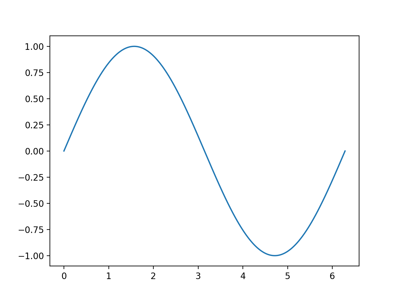
# Compare the numeric evaluation of sin to numpy's implementation in 1000 points between 0 and 2pi:
ts = np.linspace(0, 2*np.pi, 1000)
sinFromMFunc = mfn0(lambda evs: np.exp(np.outer(np.log(evs), ts/a))).coeffs
sints = np.sin(ts)
error = np.sum((sinFromMFunc - sints)**2)
print(error)
# 1.1051029979680703e-26

plt.plot(ts, sinFromMFunc)
plt.savefig('sinFromMFunc.png', dpi=200)