This tool transforms a raster containing scattered white pixels into a raster on which the area roughly defined by the scattered points is filled with white pixels. This is a filling algorithm in case the region to fill is not formally defined by specific properties of the raster. It implements a multi-scale variation of the Conway game of life.
This tools originated from the structure-from-motion field where sparse keypoints of an 3D objects appears as a set of scattered points when reprojected on images that see the objects. The objective of this tool was to have a way of extrapolating the area covered by an object on an image based on the few reporjected keypoints coming from it.
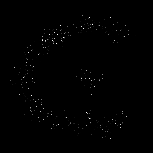
To illustrate the tools usage and results, the following example image is considered :

Original source raster contained scattered white pixels
To apply the region filling on the image, one uses the following command :
./image-morphological-conway -s example.png -e result_0.5_1.png -r 4 -f 0.5
The scale count r gives the amount of scales to consider for the process while the factor f gives the scales reduction factor that has to be between 0 and 1 (]0,1[). See the tool doxygen documentation (make doc) for more details.
The following images show the results obtained using f=0.5 and with a varying number of scales :


Process result with a reduction factor of 0.5 and 1 scale on the left and 2 on the right


Process result with a reduction factor of 0.5 and 3 scales on the left and 4 on the right
One can see how the increase of the number of scales allows to fill a greater area. This number of scales has to be adapted to the scattering of the pixels as the more scattered they are, the greater the number of scales has to be.
One can also see how the strong reduction factor of 0.5 creates sharp and squared area edges. A balance has then to be found between the quality of the edges and the filling power. In order to keep filling capacity while obtaining smoother edges, one can also play with the reduction factor value.
Increasing the factor value from 0.5 to 0.75 allows to obtain smoother edges but requires more scales to obtain the same filling capacity. One can use the following approximation of compute the new number of scale in case of a factor modification :
scale' = log( factor ^ scale ) / log( factor' )
For example, obtaining the same filling capacity of (r=3, f=0.5) with f'=0.75, one can use :
scale' = log( 0.5 ^ 3 ) / log( 0.75 ) = 7.2283 ~ 7
as the number of scale.
The following images give the results obtained with f=0.75 and a number of scales computed with the previous relation :


Process result with a reduction factor of 0.75 and 2 scales on the left and 5 on the right


Process result with a reduction factor of 0.75 and 7 scales on the left and 10 on the right
One can see how the filling capacity can be kept while obtained smoother edge on the filled area.
The following images show the results obtained with f=0.875 and a number of scale also computed with the previous relation :

Process result with a reduction factor of 0.875 and 5 scales on the left and 10 on the right


Process result with a reduction factor of 0.875 and 16 scales on the left and 21 on the right
One can see how the effect of the reduction factor affects the results. In order to obtain the desired results, one has to play with the reduction factor f and the number of scale r to obtain the appropriated balance according to the given scattered initial point set.