The Imageless Method for Spatial and Annual Glare Analysis
Author: Nathaniel L. Jones
Created: 8 September 2019
Introduction
Tutorial 1: Calculating point-in-time DGP in a computer lab
Tutorial 2: Calculating annual DGP and sGA
Tutorial 3: Calculating annual DGP using BSDFs
The “imageless method” is a means to perform annual simulation of glare caused by direct views to the sun and sky. It relies on a set of normalized coefficients (daylight coefficients) that represent flux transfer from patches of the sky to various viewing positions, where the orientation and solid angle of the sky patch with respect to each viewing position and direction is known. Daylight glare probability (DGP) under specific sky conditions is calculated by applying the sky luminance values of each patch, which are stored in a matrix with one column for each hour under consideration. Daylight coefficient and sky matrices can be calculated very quickly in comparison to the time required for rendering images of each view under each sky condition, as required by conventional glare calculation methods.
This document starts with a technical overview of the imageless method. This is followed by descriptions of glare autonomy and spatial glare autonomy, two new metrics for annual visual comfort that can be calculated quickly using the imageless method. This document also contains tutorials for using the imageless method. The first tutorial shows the calculation of DGP for many points under a single sky condition. The second tutorial shows the calculation of DGP under a range of climate-based skies and the subsequent calculation of glare autonomy and spatial glare autonomy.
This document assumes some familiarity with the basics of Radiance multi-phase methods. Users who are not familiar with them are urged to review "Daylighting Simulations with Radiance using Matrix-based Methods" by Sarith Subramaniam prior to reading this tutorial.
DGP is calculated from a brightness term using vertical eye illuminance and a contrast term that is a weighted sum of glare source luminances:
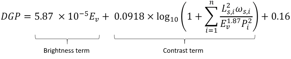
- Ev = Vertical eye illuminance
- Ls = Luminance of glare
- Ws = Solid angle of glare source
- P = Guth position index
- n = Number of glare sources
The imageless method modifies DGP by replacing the illuminance and luminance terms of the DGP equation with daylight coefficient-based calculations:


- Dtotal = daylight coefficient vector for all sky patches
- S = point in time sky luminance vector of all sky patches
- ddirect = daylight coefficient of only the direct component for sky patch i
- si = point in time sky luminance value of sky patch i
- k = 179 lumens per watt is the luminous efficacy of white light
For annual calculation, these values are stored in three matrices: Dtotal and Ddirect are created with Radiance rcontrib. The S matrix can be generated from annual weather data using Radiance genskymtx.
Given a vector of DGP values for all occupied hours for a given view, we can define glare autonomy as the fraction of time that the view is free of glare. We consider the view free of glare when DGP is below a threshold, such as 40%. Glare autonomy for multiple views can be displayed by mapping it to positions and view directions, although this typically requires the use of visualization programs outside the Radiance suite.
By setting a target for the maximum number of hours that DGP can exceed the threshold, we can also define spatial glare autonomy as the fraction of views in the space that achieve that target. Following the conventions for daylight autonomy, we abbreviate glare autonomy for a threshold of 40% DGP as GA40%, and the corresponding spatial glare autonomy with a target of 5% of occupied hours as sGA40%,5%.
Although Radiance does not pay attention to file extensions, they can be useful to the user for organizing the files used in a project. This document uses the following conventions for naming files:
| Extension | Description |
|---|---|
| *.mtx | daylight coefficient matrix |
| *.smx | sky luminance matrix |
| *.skv | sky luminance vector |
| *.ray | ray input file |
| *.dgp | output matrix of DGP values |
| *.ga | output vector of glare autonomy values |
Additionally, the following generally accepted Radiance extensions are:
| Extension | Description |
|---|---|
| *.vmx | view matrix (three-phase method) |
| *.dmx | daylight matrix (three-phase method) |
| *.xml | transmission matrix (three-phase method) |
| *.rad | radiance scene data |
| *.oct | octree file |
| *.epw | weather file (EnergyPlus format) |
| *.csv | occupancy schedule file (Daysim comma-separated value format) |
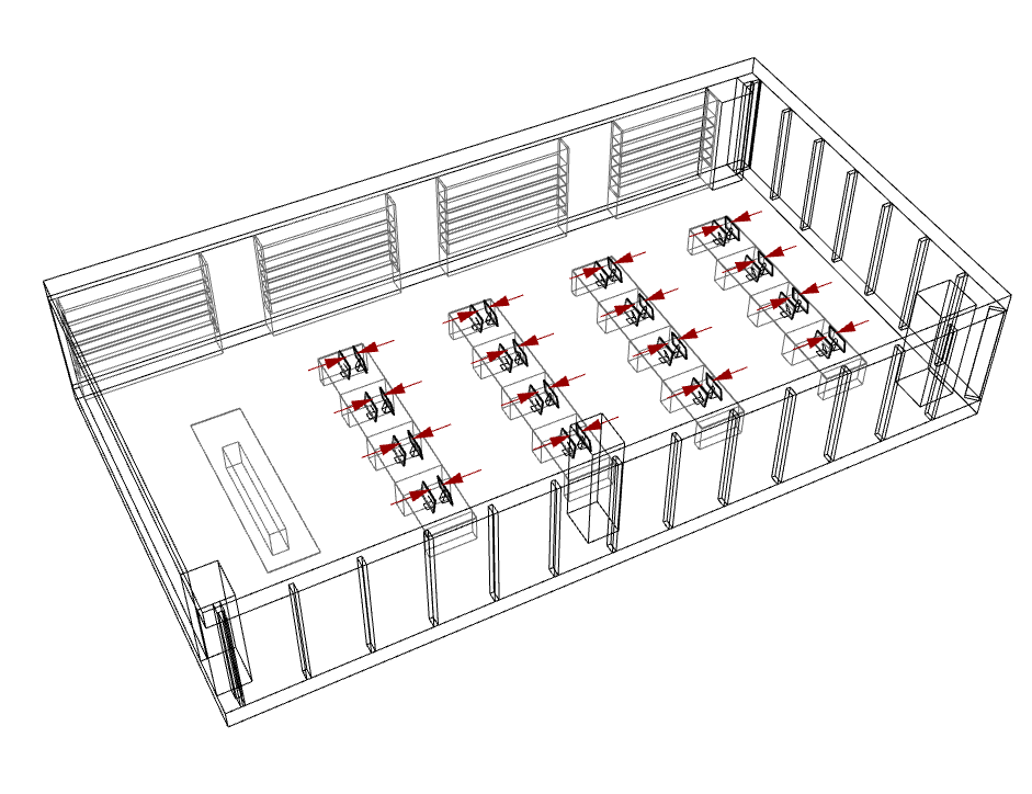
In this tutorial, we will generate a vector of DGP values for a set of views in a space at a single point in time. The views have been selected to face each screen in a hypothetical computer lab. This set of views is appropriate when the positions of occupants performing glare-sensitive tasks are known.
For this tutorial, you can download the following files:
| File | Description |
|---|---|
| computerlab.rad | the scene geometry and materials |
| uniform_sky.rad | a dummy sky that will be used to calculate daylight coefficients |
| screenviews.ray | a set of view origin points and directions corresponding to seated positions in front of each monitor |
For this example, we’ll consider a clear sky at a single point in time: 9am on December 21st in San Francisco (37.62 N, 122.40 W). The sky is discretized using the Reinhart division scheme, indicated by the -m parameter in genskyvec, where larger -m values yield higher accuracy at the expense of longer calculation times:
gensky 12 21 9 -a 37.62 -o 122.40 -m 105 | genskyvec -m 1 > skyvec_12-21-09_1.skv
gensky 12 21 9 -a 37.62 -o 122.40 -m 105 | genskyvec -m 2 > skyvec_12-21-09_2.skv
gensky 12 21 9 -a 37.62 -o 122.40 -m 105 | genskyvec -m 4 > skyvec_12-21-09_4.skv
Note that genskyvec is a Perl script. Windows users will need to replace genskyvec with perl "C:\Program Files\Radiance\bin\genskyvec.pl", using the appropriate path to the Radiance installation.
The scene description in computerlab.rad already contains all the geometry and materials needed for our calculations. However, it needs to be combined with the dummy sky and put into Radiance octree format for use by the later commands.
oconv computerlab.rad uniform_sky.rad > computerlab.octWe must create a matrix describing the direct contribution of each sky patch to each view origin point. We do this using a one-bounce ray tracing calculation. The single bounce occurs off an imaginary sensor plane that can be thought to exist at each viewing location.
Note that the Reinhart division number used here must match that of the sky vector. We will use the first division here (the Tregenza subdivision), so we use MF=1. The material name must match the material of the sky, which is sky_mat in our uniform_sky.rad file.
rcontrib -bn 1 -b "if(-Dx*0-Dy*0-Dz*1,0,-1)" -m ground_mat -f reinhartb.cal -p MF=1 -b rbin -bn Nrbins -m sky_mat -I+ -ab 1 -ad 50000 -lw .00002 -lr -10 computerlab.oct < screenviews.ray > dc1.mtxThis step differs from the previous only in that that daylight coefficients calculated here include both direct and diffuse components. We introduce the diffuse component by increasing the number of ambient bounces allowed in the calculation:
rcontrib -bn 1 -b "if(-Dx*0-Dy*0-Dz*1,0,-1)" -m ground_mat -f reinhartb.cal -p MF=1 -b rbin -bn Nrbins -m sky_mat -I+ -ab 8 -ad 50000 -lw .00002 -lr -10 computerlab.oct < screenviews.ray > dc8.mtxNow we will calculate the DGP value at each view described in screenviews.ray using the imageless substitutions into the DGP formula. This is all handled by a program called dcglare:
dcglare -vf screenviews.ray dc1.mtx dc8.mtx skyvec_12-21-09_1.skv > screenviews.dgpThe output file screenviews.dgp contains a list of 32 DGP values corresponding to the 32 views given in screenviews.ray. These can be imported into the program of your choice for visualization.
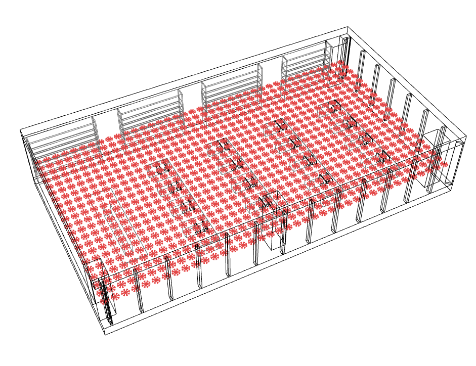
In this tutorial, we’ll perform an annual climate-based glare calculation in the same computer lab. We’ll also consider multiple view directions and a uniform grid of viewing locations. This set of views is appropriate for early stage planning when occupant locations are not yet known. Note that these two modifications could also be done independently. It is not necessary to consider multiple view directions in order to obtain annual glare metrics.
For this tutorial, you can download the following files:
| File | Description |
|---|---|
| USA_CA_San.Francisco.Intl.AP.724940_TMY3.epw | weather file for the site |
| uniformgridviews.ray | a set of uniformly distributed view positions with 8 equally-spaced viewing directions from each position |
| 8to6withDST.60min.occ.csv | occupancy schedule file in Daysim format |
We’ll expand upon the previous tutorial by using a climate-based matrix of all hourly sky conditions during the year. An hourly sky matrix contains 8760 sky vectors, including those for nighttime hours. We could edit the input EPW file or the sky matrix file to remove lines for unoccupied times in which it is not necessary to calculate glare. However, it is rarely efficient to do so. Weather files for many places on earth are available from https://app.ensims.com/epwmap.html.
Again, we can specify a Reinhart sky division for increased accuracy at the expense of a longer simulation. The default value is 1 (the Tregenza subdivision) if no -m option is provided. It is also wise to specify binary output with -of for faster file input and output.
epw2wea USA_CA_San.Francisco.Intl.AP.724940_TMY3.epw SanFrancisco.wea
gendaymtx SanFrancisco.wea > SanFrancisco_1.smx
gendaymtx -m 4 -of SanFrancisco.wea > SanFrancisco_4.smxWe will reuse the scene octree file from the first tutorial and calculate the direct and total daylight coefficient matrices as before. This time, the will be larger due to the number of points, so we again save binary files with the -faf option:
rcontrib -bn 1 -b "if(-Dx*0-Dy*0-Dz*1,0,-1)" -m ground_mat -f reinhartb.cal -p MF=1 -b rbin -bn Nrbins -m sky_mat -I+ -ab 1 -ad 50000 -lw .00002 -lr -10 -faf computerlab.oct < uniformgridviews.ray > dc1.mtx
rcontrib -bn 1 -b "if(-Dx*0-Dy*0-Dz*1,0,-1)" -m ground_mat -f reinhartb.cal -p MF=1 -b rbin -bn Nrbins -m sky_mat -I+ -ab 8 -ad 50000 -lw .00002 -lr -10 -faf computerlab.oct < uniformgridviews.ray > dc8.mtxWe can calculate DGP with the same command that we used in the previous tutorial. Note that this will calculate DGP for all sky conditions that were included in the sky matrix, including any night-time values, which will always have zero DGP.
dcglare -vf uniformgridviews.ray dc1.mtx dc8.mtx SanFrancisco_1.smx > uniformgridviews.dgpWe can also specify an occupancy schedule, which is given in the Daysim format. The schedule file should have one line for each row in the sky matrix (typically 8760 rows), and the last value on each line should be a positive value for occupied times and zero for unoccupied times. Unoccupied times will always indicate zero DGP.
dcglare -vf uniformgridviews.ray -sf 8to6withDST.60min.occ.csv dc1.mtx dc8.mtx SanFrancisco_1.smx > occupied.dgpTo calculate the glare autonomy of each view (the fraction of occupied hours in which the view is free of glare), we must provide a threshold for glare using the -l option. Note that if no schedule is given, the space will be assumed to be always occupied. For a threshold where unacceptable glare begins at 40% DGP:
dcglare -vf uniformgridviews.ray -sf 8to6withDST.60min.occ.csv -l 0.4 dc1.mtx dc8.mtx SanFrancisco_1.smx > occupied.gaThe annual DGP and glare autonomy values can be visualized using the tool of your choice.
Spatial glare autonomy will give us a single value to summarize the extent to which the space is free of glare. We will calculate the fraction of the space that exceeds 40% DGP for no more than 5% of occupied hours:
rcalc -e '$1=floor($1+0.05)' occupied.ga | total -m > spatial.gaNote that Windows users will need to use double quotes (") rather than single quotes (').
The output file spatial.ga contains a single numeric value that is the spatial glare autonomy based on the views in uniformgridviews.ray.
Coming soon...