Recommended simulation settings #2520
Comments
|
I think our default recommendation should be:
I don't think most other packages have a good sense of what to recommend and why. There seems to be a fundamental misunderstanding about what is relevant to molecular simulation, even up to the recent gromacs paper that still quantifies error in terms of drift. For sampling from configuration space, we can safely recommend BAOAB, which makes minimal error in the configuration space distribution up to the point where the integrator breaks. HMR does not perturb the configuration distribution. |
What is this referring to? I know you had issues when you were specifying a super tight tolerance like 1e-10. But a tolerance of 1e-6 is accurate enough even for most constant energy simulations, and it works fine in single precision.
Using HMR without constraining all bonds is unlikely to do much good, and can sometimes hurt. Angles that involve hydrogen and bonds that don't involve hydrogen tend to have similar frequencies. HMR slows down the former but speeds up the latter. Since the time step is limited by the fastest unconstrained degrees of freedom, this can easily mean you need a shorter time step. See https://doi.org/10.1002/(SICI)1096-987X(199906)20:8<786::AID-JCC5>3.0.CO;2-B.
It's not just a question of what's stable. Are the results sufficiently accurate for typical purposes?
According to https://dx.doi.org/10.1021/ct400109a, 1/ps has a small but non-trivial effect on dynamics and sampling. 0.1/ps mostly eliminates it, though it's still detectable. |
Yes, if you're using BOAOB: https://doi.org/10.3390/e20050318 We've found that 4 fs significantly extends the maximum stable timestep even without all-bond constraints (which is problematic because it significantly modifies the force field, especially torsion barriers). For example, for T4 lysozyme: |

|
Hm, I can't seem to find the figures that examined HMR for explicitly solvated systems using only bond constraints to hydrogens. Let me ping @maxentile to see if those are floating around somewhere convenient. It's possible I'm mis-remembering the data. |
|
Thanks for looping me in!
I haven't looked into this thoroughly enough, but a couple years ago we had looked at the effects on stability of the amber HMR scheme (scaling up the hydrogen mass and subtracting the added mass from bonded heavy atoms). We had looked at a couple different test systems (unconstrained alanine dipeptide in vacuum, and implicit-solvent T4 lysozyme with HBond-length constraints) x a few different Langevin integrators. From these initial results, it looked like the effect of H-mass scaling on stability threshold depended more sensitively on the system definition than on the choice of integrator, motivating some initial work towards developing an "auto-tuning" method that could adjust the H-mass and stepsize after the user specifies the system, integration method, temperature, collision rate, etc. For example, the stability threshold as a function of H-mass scale for AlanineDipeptideVacuum (without HBond constraints) looked qualitatively different than the one for T4LysozymeImplicit (with HBond constraints). An important caveat for the plots above: In order to have a quantity that I could precisely measure, I defined "stability threshold" in these plots as the stepsize at which half of simulations (started from equilibrium) crash within a few thousand timesteps. For a given system + collection of integrator settings, we can precisely measure this stepsize using a variant of binary search. This is also a reasonably informative quantity to measure, since the fraction of simulations that crash does appear to be a sharp threshold-like function of the stepsize for molecular mechanics models (switching from very nearly 0% to very nearly 100% as you adjust stepsize by a few hundredths of a femtosecond). However, practical stepsizes (where a user-tolerable negligible fraction of simulations crash in a production-length simulation) would be shifted lower on these plots by some amount.
I don't have analogous results for explicit-solvent systems, but could examine a few explicit-solvent testsystems using https://github.com/choderalab/thresholds if informative. |

|
I don't think the stability threshold is really the metric we want to look at. It's easy to measure, but it's also only meaningful in the sense of providing an upper limit. If the simulations blow up you know the step size is too large, but if they don't blow up the step size might still be too large to produce accurate results. Our recommended simulation settings need to balance a few goals. In order of decreasing importance:
The third one is less important than the other two because in many applications you don't care about kinetic properties. There are some where you do though. We need to figure out how to balance many different factors to best achieve these goals. And they interact in kind of complicated ways. For example:
Let me try putting together some tests of this. To start with, I'll use the same test as in #2396: simulate alanine dipeptide in a box of water and compute the average potential energy. I'll look at both the accuracy of the final answer and how quickly it converges, and see how various factors affect it. |
The point of our paper was that (1) we have a way to measure whether your simulation produces accurate results, and (2) for a wide variety of systems, if you are using BAOAB, the threshold of stability is a good surrogate to how far you can push your timestep while still getting accurate results. This should eliminate your concern above (provided we stick to recommending BAOAB). |
Which section of the paper are you referring to? I don't see where it says this. |
|
I have some preliminary results to report. First, I did some benchmarking of the cost of constraints. I ran the DHFR benchmark with the integrator being either LangevinIntegrator or BAOABLangevinIntegrator, and the constraints being either Hbonds or AllBonds. I kept everything else fixed: 2 fs time step, no HMR. Obviously you could use a larger time step with some of these settings, but I wanted to just measure the cost of computing each time step independent of that. From fastest to slowest: LangevinIntegrator, Hbonds: 414.27 ns/day So compared to the first case, switching to BAOAB is 92% as fast, constraining all bonds is 78% as fast, and doing both makes it only 52% as fast. Given that, I don't think AllBonds with BAOAB is going to be a useful combination. It would have to nearly double the step size versus Hbonds to outweigh that added computation cost. I also simulated alanine dipeptide in explicit water with BAOAB to see how various factors affect the accuracy of the ensemble. I had previously found (in agreement with published results) that increasing the step size from 1 fs to 4 fs produces a small but measurable decrease in the average potential energy, and a more significant decrease in the average kinetic energy. So I ran simulations with a 4 fs step while varying the friction and hydrogen mass. My main conclusion so far is that I probably need to run longer simulations! For my tests so far, I ran three replicates of each condition, each 1 ns long. That's enough to detect coarse changes but not smaller ones. Based on my results so far, neither friction nor hydrogen mass made a very big difference on mean potential energy. Decreasing the friction from 1/ps to 0.1/ps does seem to slow down the equilibration a little bit, but any difference on the final result is very small. It's possible that increasing the hydrogen mass leads to an increase in the potential energy, but the effect is small enough that I'm not yet totally convinced it isn't just noise. The one other significant effect is that HMR increases the observed temperature: 292K with no HMR, 295 at 2 amu, 296 at 3 amu, and 297 at 4 amu. Since the thermostat is set at 300K, this probably counts as an improvement? Though I'm not 100% certain this doesn't actually indicate an extra source of error. |
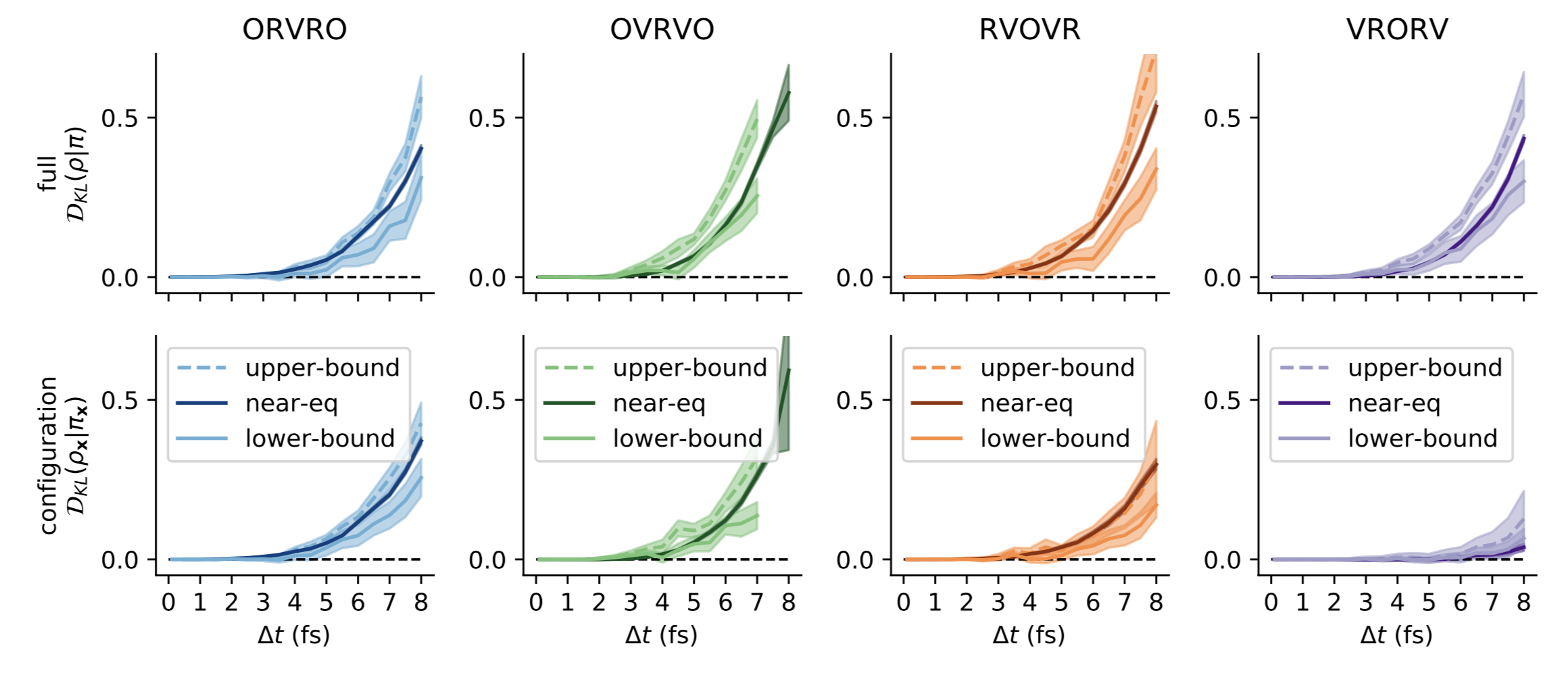
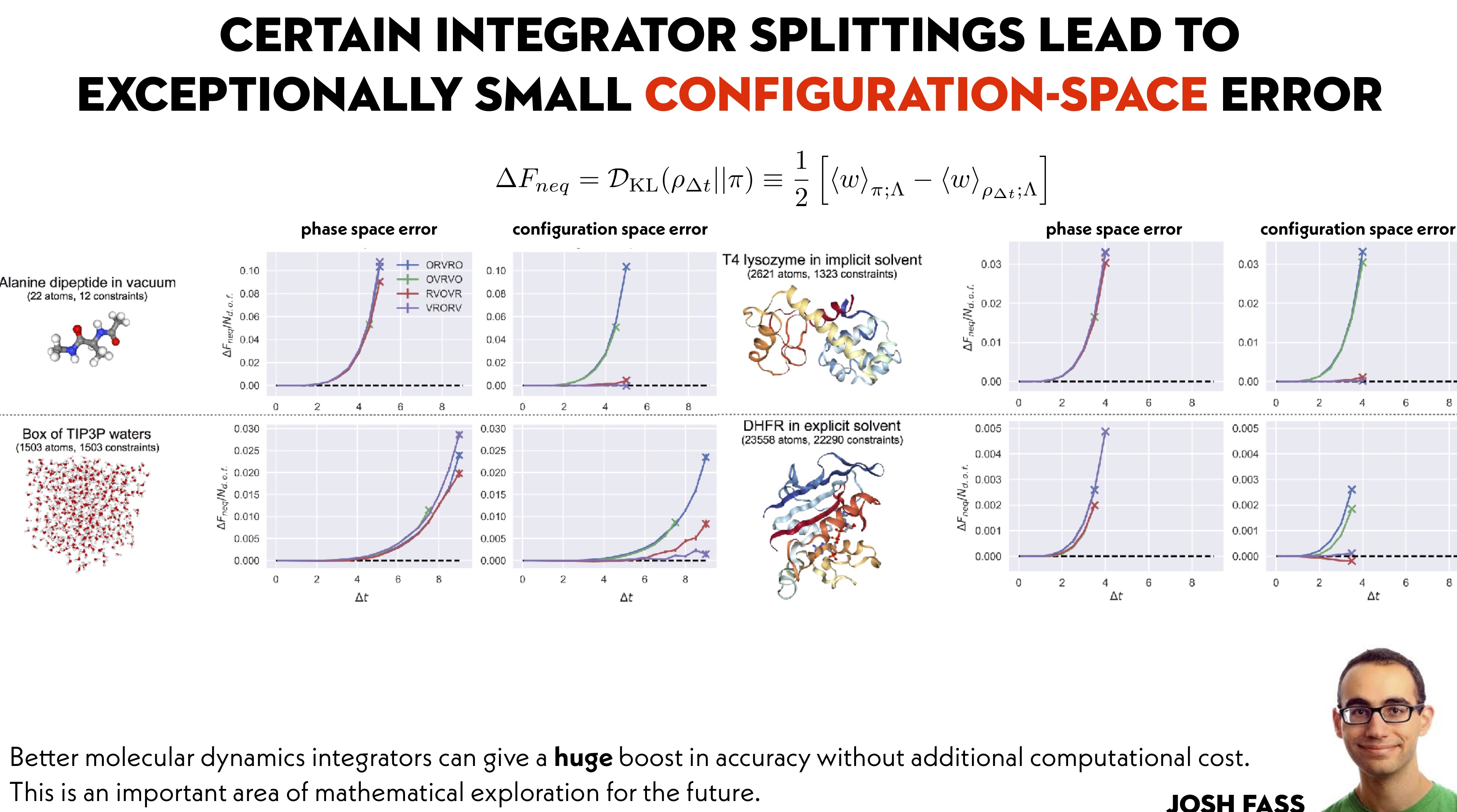
Ah! Sure thing---perhaps we could have been clearer in that take-away message (which was a main point Ben Leimkuhler was trying to make in his papers). Check out Fig 8: This is borne out in other biomolecular systems as well. In as-yet-unpublished work from @maxentile, you can see that the configuration-space error remains almost too small to measure throughout the stable timestep range (with the unstable timestep limit denoted by an X): Thanks for the great data/timings on the various integrators!
It's actually very difficult to compare the average potential energies for an explicitly solvated systems because the variance is so high and the correlation time non-trivial to estimate. Taking the stddev over three independent replicates only gives you half a digit of precision of statistical error, so it's difficult to know if the averages are statistically indistinguishable or not. We have to use careful correlation time analysis to get reliable estimates of the statistical error, but you can do that with the The "temperature" is not so meaningful here if we just care about configuration-space properties. The hallmark of BAOAB is that it pushed the integration errors from the configuration space marginals to the velocity-space marginals, but the velocity distribution is the least interesting since we know it analytically! So we tend to monitor configuration-space properties. The average potential energy includes contributions from the harmonic bonds and angles, which will be most sensitive to timestep errors, but it may also not be the most important thing for folks who want to study conformational populations. That's why we tried to develop the KL-divergence in the configuration space marginal as the most useful general yardstick for error. Or initial thinking was that if folks were willing to tolerate 2 fs timestep induced error for velocity Verlet based methods, they'd presumably be willing to tolerate the same or smaller configuration space error for BAOAB with larger timesteps. |
It also gives an estimate of the uncertainty, which is the main thing I'm after here. I also compute a standard deviation between segments of each trajectory, but that isn't always the same as what you get from independent trajectories. This way I have a pretty good idea of whether differences are significant or just noise.
True, but there are two reasons to care about kinetic quantities. First, sometimes people do simulations where they actually care about them. Second, things like increased friction or HMR can slow down sampling, which means you're not actually getting as much sampling as you think you are based on the step size. I'll do tests later to look at these more directly, for example with autocorrelation times and diffusion rates. |
That was my point: That the estimate of the uncertainty obtained from the standard deviation of three independent replicate is only precise to half a digit of precision, or one order of magnitude. So if you get 123.4 and your stderr is 0.3 from 3 replicated, you only know that the uncertainty is somewhere between 1 and 0.1, roughly speaking. You can be more precise using timeseries analysis, as I note above. |
|
And yes, for kinetic properties like transport coefficients or correlation functions, some other integrator may be better. We don't have any theory that speaks to this. But for configuration space properties, like expectations, conformational populations, and free energies, we know that BAOAB should be a best practice. |
Right, but with what time step? What friction coefficient? With or without HMR (and if with, then how much)? With what set of constraints? (I think we now have an answer for that last one.) |
|
Some of these questions are clearly system-dependent, which led @maxentile to develop this tool: https://github.com/choderalab/thresholds |
|
I have more data on this now. I ran a collection of 10 ns simulations with BAOABLangevinIntegrator in various conditions: time step of either 1 fs or 4 fs, friction of either 1/ps or 0.1/ps, and with and without HMR (setting hydrogen mass to 3 amu). For comparison, I also tested our current recommended configuration: LangevinIntegrator, 2 fs step size, 1/ps friction. Here's a plot of the mean potential energy across three replicate simulations for each one. The horizontal dotted line marks the value for 1 fs step size, 1/ps friction, which should be the closest to the "correct" result. So the distance from that line should roughly indicate the amount of error.
The results are similar to what I described before. Reducing the friction to 0.1/ps tends to make the error a little larger. Increasing the hydrogen mass makes the error a little smaller. But in all cases, the error is smaller than what we currently get with a 2 fs step size. So really, I think the error is totally acceptable for all of them. Next I wanted to look at the effect of friction and HMR on sampling. I recorded the alanine dipeptide's phi and psi angles every 100 fs and computed their autocorrelation functions. Here's the result for phi:
There's very little difference between them. They all relax quite quickly and at about the same rate. Now look at the result for psi:
This relaxes much more slowly, and there are significant differences. HMR significantly slows down the transition rate, and so does decreasing the friction coefficient. The latter is the opposite of what I expected: I thought smaller friction would produce faster transitions. But perhaps that isn't surprising, since lower friction really means weaker interaction with the heat bath. It also matches my results from the simulations to measure potential energy: lower friction leads to signficantly slower equilibration and more uncertainty in the results. The difference between phi and psi appears to reflect the differences in the energy landscape. Phi tends to move freely over almost its whole range without significant barriers, whereas psi makes less frequent transitions between distinct states that are separated by barriers. |


🎉 Nice! This result appears consistent with -- and extends on -- a result described in chapter 7 of Leimkuhler and Matthews' 2015 book. There they reported potential energy histograms of droplet-solvated alanine dipeptide for stepsize range 1-2.8fs, with collision-rate 1/ps and without constraints.
Hmm, that second conclusion is also the opposite of what I expect. If true, this would be an interesting reversal compared to what happens for alanine dipeptide in vacuum, when adjusting the collision rate over a larger range of 1e-2 to 1e+2 /ps. Compare with Figure 6 of [Leimkuhler, Matthews, 2013] "Robust and efficient configurational sampling via Langevin dynamics" https://arxiv.org/abs/1304.3269 In any case, I think recommending 1/ps probably strikes a good balance between, on the one hand, stability and configuration-sampling fidelity (which increase with friction), and on the other hand configuration-sampling exploration rate (which can dramatically slow down with increasing friction past some threshold, which may be ~1/ps for typical systems).
Finicky question: are you computing autocorrelation based on the time series of the angle itself (which occasionally might discontinuously jump between -pi and +pi) or on the sin or cos of the angle?
I also don't think there's a clear relationship between preserving the velocity marginal distribution (or summaries of it like the distribution of kinetic energies or the kinetic temperature) and preserving relevant kinetic quantities like correlation functions. Accurately reproducing the kinetic energy marginal distribution does not imply accurately reproducing other kinetic properties. For example, imagine if a program were to give you a stream of independent samples (positions, velocities) from the boltzmann distribution. The resulting velocity marginal (and thus KE marginal, and kinetic temperature) would be perfect, but any correlation time you could think to measure from that "trajectory" would be 0.... The opposite direction isn't clear either: empirically you can get some nontrivial kinetic quantities right with methods that get the kinetic-energy marginal distribution wrong (e.g. figure 6 above). |


Agreed, and that also matches https://dx.doi.org/10.1021/ct400109a which found a large slowdown for 10/ps, but only a small one for 1/ps.
It's based on the angle itself. I used the following routine to wrap everything into a consistent range: def wrap(x):
for i in range(len(x)-1):
if x[i+1]-x[i] > np.pi:
x[i+1] -= 2*np.pi
elif x[i+1]-x[i] < -np.pi:
x[i+1] += 2*np.pi
minx = x[0]
maxx = x[0]
for i in range(len(x)-1):
if x[i+1] > maxx and x[i+1] > minx+2*np.pi:
x[i+1] -= 2*np.pi
elif x[i+1] < minx and x[i+1] < maxx-2*np.pi:
x[i+1] += 2*np.pi
minx = min(minx, x[i+1])
maxx = max(maxx, x[i+1])The first loop does most of the work, but occasionally it still manages to make a jump of 2pi, so the second loop catches those cases. I visually inspected all the timecourses after wrapping to make sure they were behaving themselves properly. |
|
Thanks for posting For example, if I simulate a random walk on the unit circle, compute the resulting angle trajectory, then call My expectation is that if we inspect other autocorrelation functions, or use other estimators of this specific "transition rate", we won't find many examples where overdamped dynamics appears faster than underdamped. |
|
I reran it without the wrapping and computing the autocorrelation of the complex exponential exp(i*x) rather than x. The results are basically identical. Here is phi:
And psi:
|


I don't think it's overdamping anything. The oscillatory motions in the system (bonds, angles, impropers, peptide bonds, water librations) all have periods much shorter than 1 ps. They should only be minimally affected. At the other end of the scale, the friction coefficient of water is 91/ps. So adding an extra friction of 1/ps should have a tiny effect on any motion large enough to require bulk rearrangement of water. So this effect probably mostly applies to a limited class of motions similar to psi rotations in alanine dipeptide: ones where the sampling rate is limited by the need to cross a barrier, and which are small enough that they don't require too much water rearrangement. For example, sidechain rotations in a protein. |
|
Hmm, very interesting! I guess I always assumed that rates like that would be monotonic functions of the friction coefficient, and this seems to be hinting otherwise... If this is an important point for informing the decision of what settings to recommend, we might want to estimate barrier crossing rates rather than angle ACFs, and at a bigger grid of friction coefficients? |
|
I suspect the "right" way to answer this is to simulate a whole protein, then look at the rates of many different motions on different scales: rotations of exposed sidechains, backbone rotations in flexible regions, and so on all the way up to domain motions. That could make an interesting paper, if it hasn't already been done. Which it may well have been—we'd need to do literature search. For the present discussion though, it's probably beyond what we need to do. I suggest we go with 1/ps as the recommended value. Based on my results and on the papers cited above, that should be pretty close to optimal even if it's not exactly optimal in every case. And it makes sense as a value, since 1 ps is long compared to both internal oscillatory motions and water damping, but very small compared to the lengths of typical simulations. |
Agreed! |
|
How about the following then as our "default settings"?
That's what we'll use in our examples, and it will be the default in OpenMM-Setup. |
|
Just wanted to say that we shouldn't be creating plots like this without putting rigorous statistical error bars on them: |
|
I just spent a while fighting with LibreOffice trying to figure out how to add error bars to that plot, but eventually gave up. Anyway, the standard deviations on all those values are on the order of 10 or smaller. |
|
Matplotlib (in a Jupyter notebook) is great for this: |
|
cc @jayponder and @jppiquem whose opinions I'd very much value on this. Now that we have MTSLangevinIntegrator, which uses the BAOAB-RESPA algorithm, we need to decide what integration settings to recommend to users for AMOEBA. I've been running tests to collect data about that. Similar to the results above, I simulated alanine dipeptide in explicit solvent and computed the mean potential energy over the simulation. All simulations used no constraints, flexible water, 300 K, and 1/ps friction. I tried inner time steps of 0.25, 0.5, or 1.0 fs, and outer time steps of 2, 3, or 4 fs. I also tried two ways of splitting up the forces. The mutipoles always go in the outer time step, and the bonded forces always go in the inner time step, but the vdw forces can go in either one. To estimate the "correct" result, I also tried using a single step size of 0.5 fs for all forces. That's shown by the dotted line in the graph below. Here are the results.
The inner time step seems to make very little difference. The lines for 0.25 fs and 0.5 fs are practically on top of each other. 1.0 fs might be a little different, but it's close enough that I'm not convinced this isn't just random fluctuations. The outer time step makes more difference. The error increases steadily as the steps get larger. The thing that makes a really big difference is how the forces are split up. Putting the vdw forces into the inner step leads to much higher error. That's the opposite of what I expected. I would have thought evaluating them more often would produce less error, not more. Possibly it's relying on cancellation of error between the Coulomb and vdw forces, so evaluating them at different frequencies increases error? This still leaves the question of what is "accurate enough". What should we recommend? The differences here are quite a bit larger than the ones for point charge force fields above. In that case all results, even the ones for LangevinIntegrator, are within 100 kJ/mol of the correct result. In this case, the differences between conditions are an order of magnitude larger. But maybe they're just not comparable. In addition to using a different force field, those simulations used rigid water and hbond constraints, while these ones are fully flexible, so there are a lot more degrees of freedom. |

|
@peastman : Thanks for doing this analysis! @maxentile and I put out a paper that I feel is the current best practice for assessing integrator error for Langevin-type integrators. In it, we measure the error introduced into the configuration-space probability density that is sampled. While this does not directly allow you to compute the error in any given property of interest---such as protein-ligand binding affinities---ensuring configuration-space error is low will guarantee errors remain low in those properties. Here is an example of what this looks like for a simple model system:
An important consideration is that we should be comparing not to the 0.5 fs timestep, but rather the exact Monte Carlo result. @maxentile has some hybrid Monte Carlo integrators we may be able to use to generate these exact samples from the desired distribution. Typically, he generates an (expensive) set of uncorrelated samples with HMC and then uses the same set of samples as reference for evaluating the KL-divergence with short trajectories without Metropolization. One question about the splitting used in this experiment: When you talk about splitting "vdW"---what do you do with the vdW and electrostatics exceptions? Do they get bundled into the valence terms in the inner timestep, or the nonbonded interactions in the outer timestep? |

|
My initial impression is the results in Peter Eastman's 2-3-4 fs/inner-outer plot above appear to confirm what I've decided over many years of playing with multiple time step integrators. My conclusion has always been that if you only use two time step ranges in the splitting, and put all of each individual term into either the inner or outer step as this new integrator is doing, then the best you can do "safely" is a 2 fs outer time step. We have had our standard Tinker "RESPA" two-stage integrator that uses 0.25 fs inner and 2.0 fs outer, with electrostatics and vdw in the outer, in the C++ interface of "Tinker-OpenMM" for years. That integrator is what Pengyu Ren's group and my group have used for all of our AMOEBA simulations, including free energy calculations. It is rock-solid stable. Sorry to be a pessimist, but my intuitive guess without you doing any kind of detailed statistics is that the errors shown for the 3 fs and 4 fs outer steps are too big for lots of "careful" work... I think the only way to really get much better overall throughput/efficiency is to move to at least three, and perhaps four, time step ranges. |
|
Hi all, we published a paper dedicated to AMOEBA last year, exactly in this topic. Pushing the limits of Multiple-Timestep Strategies for Polarizable Point Dipole Molecular Dynamics L. Lagardère, F. Aviat, J.-P. Piquemal, J. Phys. Chem. Lett., 2019, 10, 2593−2599 DOI: 10.1021/acs.jpclett.9b00901 |
|
Doing the three way split in your paper would be difficult. The multipole code in OpenMM would need changes if we wanted to be able to split it into short and long range parts. I believe the splitting above is identical to what you call BAOAB-RESPA in your paper? The paper implies (though it may not explicitly state) that a 3 fs outer step is acceptable with that splitting. Also, your tests all use a 0.25 fs inner step. As far as I can tell, no other size was considered. From my results above, 0.25 fs has no advantage over 0.5 fs, and possibly not even over 1 fs. How was that size chosen?
Yes, but the hard problem is the one we need to solve. :) It's very easy to say that a 2 fs outer time step is more accurate than 3 fs. But is 3 fs still accurate enough? If not, what about 2.5 fs? We need some objective measure for deciding. |
|
Using a 3 fs outer step for the simple two-range bonded-nonbonded BAOAB-RESPA integrator is kind of marginal, in my opinion. It perturbs properties, including the diffusion of water being 6% low, etc. As you start to damp the dynamics, you are essentially fooling yourself in the sense that your "sampling power" will be lower than what the gross simulation time in ns would suggest. Hydrogen mass repartitioning (HMR) also damps dynamics. With the above said, the further RESPA1 splitting, originally suggested by Tuckerman and used in J-P's paper for the stochastic BAOAB-RESPA1 method is a very good thing. However, as Peter suggests it is more work to implement multi-stage splittings, and especially when a single energy term is distributed across several time ranges. As to the inner step for bonded interactions, lots of tests were run a long, long time ago (10+ years) when simple Newtonian two-range Verlet-RESPA was first implemented in Tinker. As I recall 0.25 fs is essentially "perfect" in that nothing changes if you go even smaller-- I think I may have actually tried 0.1 fs. An inner step of 0.5 fs is pretty good, and in my hands a step of 1.0 fs was then much worse. We went with 0.25 fs instead of 0.5 fs in Tinker "out of an abundance of caution", and because the overall speed savings on CPUs between 0.25 and 0.5 was quite small. |
|
@jayponder brings up a great point: Is the goal to accurately and efficiently sample the configuration distribution (e.g. for binding free energy calculations) or accurately model kinetics? For sampling the configurational distribution, @jayponder is right that HMR and other tricks may perturb the dynamics, but the key is to look at the statistical inefficiency for generating uncorrelated samples in properties of interest (e.g. the instantaneous density, water expulsion from a binding site to permit ligand binding, diffusion in alchemical space, the correlation time of dU/dlambda for TI, etc.). It's very possible that the impact on these correlation times may be minimal. |
|
I'm running more tests to reduce the error bars and get a clearer sense of the impact of the inner time step. Hopefully using BAOAB will at least let us make that larger. I'll post the results when they finish. Doing a three way split is going to have to wait. Once 7.5 is released, I'd like to do a major overhaul of the AMOEBA code. I'll open a separate issue to discuss that. |
|
Here are the average energies from a set of longer simulations. These all had an outer step of 2 fs while varying the inner step. 0.25 fs: -26853 +/- 36 All these values are statistically indistinguishable from each other, and also from my previous numbers which were based on shorter simulations. So it looks to me like with BAOAB, 1 fs is fine for the inner time step. |
|
#927 is also relevant for this discussion |
|
I think everything in this issue is now resolved. We've selected recommended settings, updated the manual and examples, and updated the benchmark script. So I think it can finally be closed! |
|
Are there also recommended settings for the implicit solvent? The benchmarks.py still uses |
|
This issue is talking about integrator settings, because we introduced a new integrator. It applies to all force fields, which haven't changed. 91/ps is correct if you want accurate kinetics. If you just want conformational sampling, reducing it to 1/ps will do it much more efficiently. |
|
At the moment, the current settings: Usually work well with solvable proteins, but fail very often with membrane embedded proteins. I have to increase HMR to 3 or 4, which usually works. Usually the bigger is the membrane protein and the smaller is the lipid patch, the more problems do I have. For example -> 40 aminoacid protein in a lipid membrane -> HMR to 2-3. 200 aminoacid protein in a lipid membrane -> problems are starting to appear, but HMR 3-4 works. 400 aminoacid protein in a lipid membrane -> I have to heavily tune the settings to not a system explosion |
|
Thanks for the report! Would you be willing to submit a ZIP archive of a
couple of the more difficult systems so we could explore some alternative
automated options? The PDB/CIF input file with the script you use to read
and apply force field parameters should be sufficient.
|
When I will get out from the pile of university's paperwork, I will try to gather few examples that I have to. Now I'm under a rain of documents |
Now that we have BAOABLangevinIntegrator, we should think about updating our recommended simulation settings. These settings come up in lots of places:
Currently we have two sets of recommended settings:
If we want to start recommending BAOABLangevinIntegrator instead, we need to select settings to recommend with it. We can presumably increase the time step (to make the simulation run faster), decrease the friction (to make sampling more efficient), or both. What values can we use while still only constraining hbonds? Is there still value in also recommending settings with AllBonds? Is HMR useful, or does that only help when using AllBonds?
We should look at what settings are recommended with other programs, but also run our own tests.
The text was updated successfully, but these errors were encountered: