Team

Feli Gentle	Tyler Woods	Wesley Nguyen

Table of Contents

• Overview
• Exploring Data
  • Initial Intake
  • Feature Engineering
  • Visualizations
• Predictive Modeling
  • Baseline
  • Evaluation
  • Tuning
• Performance
• Future Considerations
• License
• Credits
• Thanks

Overview

Main Goal:
Predicting the sales price of a particular piece of equipment at auction, based on it's usage, equipment type, and configuration, and other available features.

Business Context:
Whether you're buying, selling, or analyzing market dynamics, predicting sales prices is a valuable insight for a business.

When analyzing a business's own inventory, a reliable price prediction model can inform annual budgets and projected revenue. Additionally, the information gained sheds light on what it is about an item that tends to have the biggest impact on sale price at auction time. Knowing these features can inform a business on how to build and maintain an inventory that holds value over time.

Knowing the projected prices of other business's items can inform what a fair market value is when growing one's inventory. This insight can additionally help with budgeting and negotiation when purchasing.

Let's look further at how we built our predictive model.

Note: This data consists of data from auction postings and sales prices. It includes information on the usage and specifications of the machinery.

Evaluating Success:
The evaluation of our model will be based on Root Mean Squared Log Error.
Which is computed as follows:

where p_i are the predicted values (predicted auction sale prices) and a_i are the actual values (the actual auction sale prices).

Exploring Data

Initally going into this case study, we decided to tackle the tasks of cleaning the data, and getting a baseline model together as a group. We did this to ensure that everyone was on the same level of understanding before we delved into partitioned tasks.

Initial Intake

Initial Data

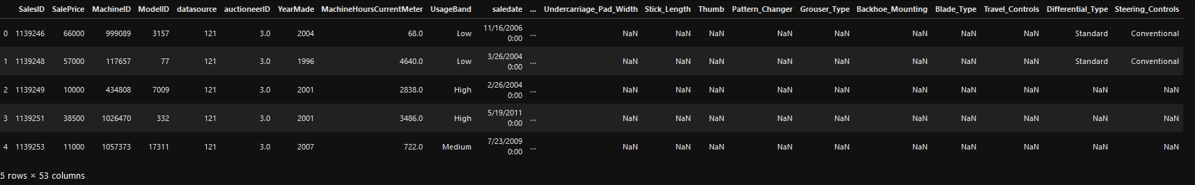
Cleaning Data: With the intent of using Linear Regression in mind, we processed and cleaned some of the data in order for this to be possible. Using a custom function, we dropped rows that had a high percentage of null values.

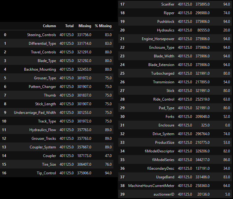
Columns with more than 50% Missing Values

df.drop(columns=['UsageBand','Blade_Extension', 'Blade_Width', 'Enclosure_Type',
                     'Engine_Horsepower', 'Pushblock', 'Scarifier', 'Tip_Control',
                     'Coupler_System', 'Grouser_Tracks', 'Hydraulics_Flow','Backhoe_Mounting', 
                     'Blade_Type', 'Travel_Controls','Differential_Type','Steering_Controls',
                     'SalesID','fiBaseModel','fiSecondaryDesc',
                     'fiModelSeries','fiModelDescriptor', 'auctioneerID',
                     'Drive_System', 'datasource'
                    ], inplace=True)

Product Size	Ripper Values

Feature Engineering

Cleaning Functions:

def getNullCount(df:pd.DataFrame) -> None:
    """Prints metrics of null values from a dataframe"""
    columns = df.columns
    for col in columns:
        total_nan = sum(pd.isna(df[col]))
        total_all = df[col].size
        print(f"Column: {col}  Total:{total_all}  Missing:{total_nan}  {round(total_nan/total_all, 2) * 100}%")

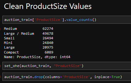
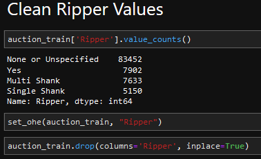
# One Hot Encode Categoricals
def set_ohe(df:pd.DataFrame, col_name:str) -> None:
    """One Hot Encodes Dataframe column"""
    for val in auction_train[col_name].value_counts().index:
        df[f"{col_name}: {val}"] = df[col_name].map(lambda x: 1.0 if x==val else 0.0)

One Hot Encoding: We noticed that there were groupings of items within certain columns and decided to use OHE to convert these values to binary values.

Cleaned Data

Visualzations

---

Predictive Modeling

Baseline

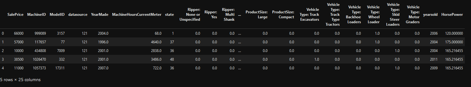
Baseline Model: Linear Regression

We started out using a Linear Regression as a baseline model to start with, and then figure out where to go from there.

# Split up Data Between Features (X) and SalePrice, i.e. the Target Values (y))
X = clean_df.drop(columns=['SalePrice'])
y = clean_df['SalePrice']

summary_model(X, y)

OLS Summary

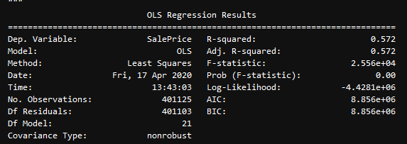
# Split up Data Between Features (X) and SalePrice, i.e. the Target Values (y))
X = clean_df.drop(columns=['SalePrice'])
y = clean_df['SalePrice']

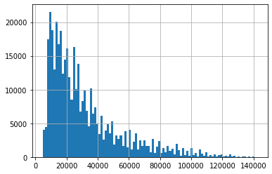
y.hist(bins=100)
plt.show()

To get a sense of what the distribution of our target values were, we plotted it in a histogram

Sales Price Histogram

# Split up Data Between Features (X) and SalePrice, i.e. the Target Values (y))
X = clean_df.drop(columns=['SalePrice'])
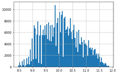
# Log the Target
y = np.log(clean_df['SalePrice'])

y.hist(bins=100)
plt.show()

As seen below, the distribution of the target values are bunched to the left, so we needed to find a way to center the mean in order to create a more accurate model

Sales Price Histogram (Log)

RMSLE: Cross Validation Errors (Pre-Log)

n_folds = 10
kf = KFold(n_splits=n_folds, shuffle=True)
test_cv_errors, train_cv_errors = np.empty(n_folds), np.empty(n_folds)
X_array = np.array(X)
y_array = np.array(y)

for idx, (train, test) in enumerate(kf.split(X)):
    model = LinearRegression()
    model.fit(X_array[train], y_array[train])
    y_hat = model.predict(X_array[test])
    y_train = model.predict(X_array[train])
    
    train_cv_errors[idx] = rmsle(y_array[train], y_train)
    test_cv_errors[idx] = rmsle(y_array[test], y_hat)

train_cv_errors, test_cv_errors

(array([15049.50547112, 15077.59371394, 15064.28882563, 15064.36987342,
        15070.18482936, 15076.58622347, 15073.01997752, 15054.20483307,
        15063.71687785, 15065.55533862]),
 array([15214.63656495, 14961.68865696, 15081.91996435, 15081.54609959,
        15028.80838643, 14971.77556378, 15003.28669371, 15172.473795  ,
        15086.84958932, 15070.36424814]))

RMSLE: Cross Validation Errors (Post-Log)

n_folds = 10
kf = KFold(n_splits=n_folds, shuffle=True)
test_cv_errors, train_cv_errors = np.empty(n_folds), np.empty(n_folds)
X_array = np.array(X)
y_array = np.log(np.array(y))

for idx, (train, test) in enumerate(kf.split(X)):
    model = LinearRegression()
    model.fit(X_array[train], y_array[train])
    y_hat = model.predict(X_array[test])
    y_train = model.predict(X_array[train])
    
    train_cv_errors[idx] = rmsle(y_array[train], y_train)
    test_cv_errors[idx] = rmsle(y_array[test], y_hat)

train_cv_errors, test_cv_errors

(array([0.03681113, 0.03676828, 0.03682234, 0.03681786, 0.03676724,
        0.03680314, 0.03682065, 0.0368372 , 0.03679243, 0.0367921 ]),
 array([0.03673228, 0.03713358, 0.03661953, 0.03666285, 0.03713166,
        0.03680484, 0.03665091, 0.03649925, 0.03690903, 0.03691538]))

Evaluation

OLS Summary on Features

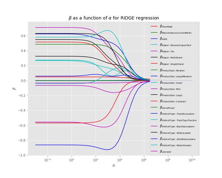
Ridge Regression

We decided that using a Ridge Regression would be the best model for this situation in order to find out which features would be most important.

y = np.array(clean_auction['SalePrice'])
X = np.array(clean_auction.drop(columns='SalePrice'))

X_train, X_test, y_train, y_test = train_test_split(X, y)

model = Pipeline([('standardize', StandardScaler()),
                   ('regressor', Ridge())])

model.fit(X_train, y_train)

Tuning

---

Performance

Model Prediction

y_hat_train = model.predict(X_train)
y_hat_test = model.predict(X_test)

print('Training error: {}'.format(rmsle(y_train, y_hat_train)))
print('Testing error: {}'.format(rmsle(y_test, y_hat_test)))

Training Error:	Testing Error
0.0368246720958709	0.03672861629228472

Using data from the file data/test.csv, we used our model to obtain an RMSLE of 0.573.

Note: The best RMSLE was only 0.23 (obviously lower is better). Note that if you were to simply guess the median auction price for all the pieces of equipment in the test set you would get an RMSLE of about 0.7.

Interpreting our Results

This root mean squared log error signifies that our model predicts a sale price that is within 1 order of magnitude of the actual price. Although there is plenty of room for improvement, we're able to get 'in-the-ballpark' of the sale price, so that our customer will have an idea of how much their heavy machinery will sell for.

Future Considerations

Cleaning the data and finding the important columns was the biggest hurdle. We decided to do one-hot-encoding for multiple columns of the dataset and drop most of the other columns.

Once we felt that we had a data set that was cleaned and ready, using different models was quick.

License

MIT ©

Credits

Thanks