OpenCV + Machine Learning
- Make sure to have the correct xml file content and path for cascade detector.
- Points in openCV are defined in the order of (X, Y), but matrix is in the order of (nRow, nCOl).
- The best way to define points in openCV is in
tuple. Convertnumpy.array.tolist()to list and then to tuple before feeding into openCV functions. - The transformation matrix
cv2.warpAffine()lists in the order of (X, Y). - To shrink an image, it will generally look best with cv2.INTER_AREA interpolation, whereas to enlarge
an image, it will generally look best with cv2.INTER_CUBIC (slow) or cv2.INTER_LINEAR (faster but still looks OK). Finally, as a general rule, cv2.INTER_LINEAR interpolation method is recommended as the default for whenever you’re upsampling or downsampling — it simply provides the highest quality results at a modest computation cost.
- Flipping operations could be very useful in augment dataset (flipping images of faces to train machine learing algorithms)
- There is a difference between OpenCV and NumPy addition. NumPy will perform modulus arithmetic and “wrap around.” OpenCV, on the other hand, will perform clipping and ensure pixel values never fall outside the range [0, 255].
cv.addbehavior:
>>> cv2.add(np.uint8([10]), np.uint8([250]))
array([[255]], dtype=uint8)
>>> cv2.add(np.uint8([10]), np.uint8([260]))
array([[14]], dtype=uint8)
- Cropping can be realized through slicing numpy arrays, and also bitwise operations. Irregular cropping other than rectangular one can only be realized using bitwise operations.
- For simple masking,
cv2.bitwise_and(image, image, mask=mask) cv2.splitandcv2.mergeare convenient functinos to convert between 3ch color and 1ch graysale images.- Global image classification and local object detection are two distinctive topics in computer vision. The latter can be seen as a special case of the former (when the bouunding box or image size is sufficiently small).
- An object is what can be represented as a semi-grid structure with noticeable patterns. Objects in real world have substantial variations which makes classification and detection difficult (e.g., viewpoint, deformation, occulusion, illumination, background clutter, intra-class variation, etc).
- template matching is the simplest form of object detection technique. The template must be nearly identical to the object to be detected for this technique to work.
- In template matching, the matching method is very critical. Generally
cv2.TM_CCOEFFgives good results. - dlib is a cross platform computer vision library written in C++. It is best used to train object detection.
- Training an object detector is very similar to training a classifier to (globally) classify the contents of an image, however, both the labels of the images and annotations corresponding to the bounding box surrounding each objectare needed. Features could be extracted from the bounding boxes, and then used to build our object detector.
- .mat files in Matlab are serialized, like .pickle files in python. Pickling is a way to convert a python object (list, dict, etc.) into a character stream. The idea is that this character stream contains all the information necessary to reconstruct the object in another python script.
- kernels are used with convolution to detect edges
- Smoothing and blurring is one of the most common pre-processing steps in computer vision and image processing
- Applying Gaussian smoothing does not always reduce accuracy of object detection. It is generally suggested to run two experiemnts, one with and one without Gaussian filter and pick whichever gives better accuracy. It is shown that applying Gaussian filter at each layer of the pyramid can actually hurt the performance of the HOG descriptor — hence we skip this step in our image pyramid.
- Use generator
yieldto create pipeline if there is too much data involved. - Choosing an appropriate sliding window size is critical to obtaining a high-accuracy object detector.
- When there is a lot of parameters to be passed to a command line tool, it is best to design a JSON file to store all the parameters.
virtualenv in iPython notebook link
- Install the ipython kernel module into your virtualenv
workon my-virtualenv-name  # activate your virtualenv, if you haven't already
pip install ipykernel
- Now run the kernel "self-install" script:
python -m ipykernel install --user --name=my-virtualenv-name
Replacing the --name parameter as appropriate.
- You should now be able to see your kernel in the IPython notebook menu: Kernel -> Change kernel and be able so switch to it (you may need to refresh the page before it appears in the list). IPython will remember which kernel to use for that notebook from then on.
cv2.getRotationMatrix2D(center, angle, scale)cv2.warpAffine(src, M, dsize)
A basic explanation can be found here and here on stack exchange and in this ppt, which includes 4 major steps.
-
Preprocessing:
- RGB-> YCbCr space; 2x subsampling of chroma components leads to 2x compression (1+1/4+1/4 = 1.5 = 3**/2**).
- Partitioning into 8x8 blocks;
- subtract 127
-
Transformation: Discrete Cosine Transformation (DCT);
Loosely speaking, the DCT tends to push most of the high intensity information (larger values) in the 8 x 8 block to the upper left-hand of C with the remaining values in C taking on relatively small values. C = U B U^T.
DCT is reversible. DCT coefficients can be viewed as weighting functions that, when applied to the 64 cosine basis functions of various spatial frequencies (8 x 8 templates), will reconstruct the original block.
-
Quantization. This step leads to information loss.
-
Encoding:
- Zigzag ordering
- Huffman encoding
- BGR is used in openCV for historical reasons.
- BGR images are stored in a row-major order
- Kernel visualization tool
- Sobel filters are directional. Left Sobel filter is different from right Sobel filter, also both are veritical Sobel filters. When both edges need to be detected, it is better to keep data type to higher forms, take abosolute value and conver back to np.uint8 or cv2.cv_8U.
- Structuring elements are similar to kernels, but not used in the context of convolution.
- Intro to morphological operatinon link
- The white top-hat transform returns an image, containing those "objects" or "elements" of an input image that:
- Are "smaller" than the structuring element (i.e., places where the structuring element does not fit in), and
- are brighter than their surroundings.
- The black top-hat (or black hat) returns an image, containing the "objects" or "elements" that:
- Are "smaller" than the structuring element, and
- are darker than their surroundings.
- In other words, top hat returns features that would be eroded; black hat returns features that would be dilated.
- Median filter is nonlinear and best at removing "salt and pepper" noise, and creates "artistic" feeling as the image would appear blocky. Median filter will remove substantially more noise. Gaussian blur appears more natural.
- Bilateral filtering considers both the coordinate space and the color space (domain and range filtering, ergo bilateral). Only if the neighboring pixel's value is close enough will it be contributing to the blurring of the pixel of interest. This will selectively blur the image and will not blur the edges. Large filters (d > 5) are very slow, so it is recommended to use d=5 for real-time applications, and perhaps d=9 for offline applications that need heavy noise filtering. (perhaps meitu used it for remove wrinkles!)
- In both Gaussian blur and bilateral filtering, there are two parameters, d and sigmaSpace that controls behavior in the coordinate space. It is the best practice to specify both. d is the finite (truncated) support of an infinite Gaussian surface with sigmaSpace.
- The camera is not actually “filming” the object itself but rather the light reflected from our object. The success of (nearly) all computer vision systems and applications is determined before the developer writes a single line of code. Lighting can mean the difference between success and failure of your computer vision algorithm. The quality of light in a given environment is absolutely crucial, and perhaps the most important factor in obtaining your goals. You simply cannot compensate for poor lighting conditions.
- The ideal lighting condition should yield high contrast in the ROI, be stable (with high repeatability) and be generalizable (not specific to a particular object).
- It is extremely important to at least consider the stability of the lighting conditions before creating a computer vision system.s
- RGB: Most popularly used. Additive color space, but color definition is not intuitive.
- HSV:
- HSV is much easier and more intuitive to define a valid color range using HSV than RGB.
- The HSV color space is used heavily in computer vision applications — especially if we are interested in tracking the color of some object in an image.
- Hue: how pure the color is
- Saturation: how white the color is. Saturation = 0 is white, while fully saturated color is pure.
- Value: lightness, black to white
- L*a*b*:
- The Euclidean distance between two arbitrary colors in the L*a*b* color space has actual perceptual meaning.
- It is very useful in color consistency across platforms, color management.
- The V(alue) channel in HSV is very similar to the L-channel in L*a*b* and to the grayscale image.
- Grayscale: Grayscale is often used to save space when the color information is not used. Biologically, our eyes are more sensitive to green than red and then than blue. Thus when converting to grayscale, each RGB channel is not weighted uniformly:
$$Y = 0.299 \times R + 0.587 \times G + 0.114 \times B$$ Human beings perceive twice green than red, and twice red than blue. - Note that, grayscale is not always the best way to flatten image to a single channel. Sometimes, convert to HSV space and then use V can yield better results.
- HDF5 is a binary data format that aims at facilitating easy storage and manipulation of huge amounts of data. HDF5 is written in C, but can be accessed through
h5pymodule. When using HDF5 withh5py, you can think of your data as a gigantic NumPy array that is too large to fit into main memory, but can still be accessed and manipulated just the same.
- To mask the object in a white background, use
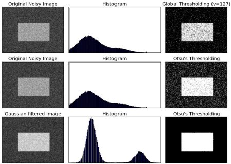
cv2.THRESH_BINARY_INV. - Otsu's method assumes a bi-modal distribution of grayscale pixel values. Otsu's method works best after Gaussian blur, which helps to make the histogram more bimodal.
- While using Otsu's method to find threshold, specify the threshold to 0 and supply additional
cv.THRESH_OTSUto options:cv2.THRESH_BINARY_INV | cv2.THRESH_OTSU
- While using Otsu's method to find threshold, specify the threshold to 0 and supply additional
- Adaptive filtering: scikit-image has a function
skimage.filters.threshold_adaptive()orskimage.filters.threshold_local()link, which has more powerful options thancv2.adaptiveThreshold()link
-
We use gradients for detecting edges in images, which allows us to find contours and outlines of objects in images. We use them as inputs for quantifying images through feature extraction — in fact, highly successful and well-known image descriptors such as Histogram of Oriented Gradients (HOG) and SIFT are built upon image gradient representations. Gradient images are even used to construct saliency maps, which highlight the subjects of an an image.
-
Image with detected edges are generally called edge maps.
-
Gradient magnitude and orientation make for excellent features and image descriptors when quantifying and abstractly representing an image.
-
Scharr kernel may give better approximation of the gradient than Sobel kernel.
Scharr = [[+3, +10, +3], [0, 0, 0], [-3, -10, -3]] Scharr = [[+1, +2, +1], [0, 0, 0], [-1, -2, -1]] -
The magnitude and orientation of the gradient:
 mag = np.sqrt(gX ** 2 + gY ** 2)
 orientation = np.arctan2(gY, gX) * (180 / np.pi) % 180
Note that
gXandgYshould be in signed float. If we wish to visualizegX, we can usecv2.convertScaleAbs(gX)to convert signed float to unsigned 8-bit int. openCV docs
- Canny edge detection entails four steps:
- Gaussian blur
- Sobel x and y gradients
- Non maximum suppression
- Hysteresis thresholding
- The optimal value of the lower and upper boundaries of the hysteresis thresholding in Canny detection
cv2.Canny(image, lower, upper)varies from image to image. In practice, setting upper to 1.33 * image medium and lower to 0.67 * image medium yields very good results. Remember the magic number sigma=0.33.
-
Contours can sometimes replace machine learning at solving some problems efficiently.
-
For better contour extraction accuracy, it is preferable to use binary image rather than grayscale image.
-
It is more productive to use
cv2.drawContours()to draw all contours while slicing the contour list, rather than specifying the contour index, i.e.,cv2.drawContours(clone, cnts[:2], -1, (0, 255, 0), 2) -
Use contour mask and bitwise_and to extract each shape in the image.
mask = np.zeros(clone.shape, dtype=np.uint8) cv2.drawContours(mask, [c], -1, 255, -1) cv2.imshow("Image + Mask", cv2.bitwise_and(clone, clone, mask=mask)) -
Contour properties: Standard bounding box is used a lot more than rotated bounding box. Minimum enclosing circle or fit ellipse are relatively rarely used. Arc length and area are used very often for contour approximation.
-
Aspect ratio:
aspect ratio = image width / image height. Aspect ratio is very effecitve in detecting certain objects. For example, most digits and characters on a license plate have an aspect ratio that is less than 1. The license plate itself is an example of a object that will have an aspect ratio greater than 1. Squares and circles are examples of shapes that will have an aspect ratio of approximately 1.
cv2.calcHist()can be used to calculate 1D or multi-dimensional histograms and more powerful thanplt.hist().- When plotting multi-dimensional hitograms,
- Connected component analysis is performed on binary or thresholded images.
- In openCV (cf link), use
cv2.connectedComponentsWithStats()orcv2.connectedComponents(). Alternatively, in scikit-image, useskimage.measure.label().
- Haralick features, or texture features, can be used to describe image texture.
- HOG + Linear SVM is superior to Haar Cascade (Viola-Jones Detector):
- Haar cascades are extremely slow to train, taking days to work on even small datasets.
- Haar cascades tend to have an alarmingly high false-positive rate (i.e. an object, such as a face, is detected in a location where the object does not exist).
- What’s worse than falsely detecting an object in an image? Not detecting an object that actually does exist due to sub-optimal parameter choices.
- Speaking of parameters: it can be especially challenging to tune, tweak, and dial in the optimal detection parameters; furthermore, the optimal parameters can vary on an image-to-image basis!
- HOG + Linear SVM entails 6 steps:
- Obtain positive examples by extracting HOG features from ROIs within positive images
- Obtain negative examples by extracting HOG features from negative images
- Train linear SVM.
- Obtain hard negative examples by collecting false positives on negative images
- Train linear SVM using hard negative mining (HNM) to reduce false positive rate.
- Non maximum suppression (NMS) to select only one bounding box in one neighborhood.
- It should be noted that the above steps could be simplified by obtaining positive AND negative examples from the ROI and other parts of the training positive images, respectively. This is implemented in
dliblibrary.
- Data preparation
- Feature extraction
- Detector training
- Non-maxima suppression
- Hard negative mining
- Detection retraining
-
Two most important parameters in HOG descriptor are
pixel_per_cellandcell_per_block. -
It’s very common to have your
pixels_per_cellbe a multiple of four. Thecells_per_blockis also almost always in the set {1, 2, 3} -
If we have N*M image,
pixel_per_cellis (n, m), andcell_per_blockis (c, c) (where c = 1, 2, or 3),orientationsis k, then the total number of features is((N/n + 1 - c) * c * (M/m + 1 - c) * c ) * k = (N/n + 1 -c) * (M/m + 1 - c) * c * c * k
For example, we have image patches of 96*64, (4, 4) pixels per cell, (2, 2) cells per block, n_orientation is 9, then total number of features is (96/4+1-2)(64/4+1-2) * 2 * 2 * 9 = 12420.