Lucius LTV

A Python simple multi-cohort LTV calculator library for subscription-based products.

Installation

pip install lucius-ltv

Building a cohort matrix

To use this library, the first step is to build a Cohort retention matrix for your product.

To build a cohort matrix:

• For each period of interest (week/month/year - depending on your subscription)
• Retrieve the number of users that started paying for the first time
• Track those users over time to observe how many where still alive in the following periods
• Stack them in order to obtain a pd.DataFrame resembling this:

2022	2021	2020	2019	2018	2017	2016	2015
100	95	82	78	75	71	68	63
	120	109	99	87	80	67	66
		101	90	80	77	73	68
			130	122	115	108	99
				95	91	85	67
					102	90	81
						90	80

Alternatively if you are just trying out this library, you can generate a retention cohort matrix by calling generate_synthetic_cohort_matrix. An example of this is contained in the sample file, sample.py shipped with this project.

Fitting the model

Once you have a cohort matrix, you can finally fit the sBG model that will predict LTV. Behind the scenes this library implements "Fader, Peter and Hardie, Bruce, How to Project Customer Retention (May 2006)" (Available at SSRN: https://ssrn.com/abstract=801145 or http://dx.doi.org/10.2139/ssrn.801145) using the powerful Bayesian Inference library pymc3.

To fit the pymc model, simply run:

Basic fit

inference_data, model = fit_sbg_model(
    cohort_matrix,
    periods=10,    # Number of projected periods
)

Fit with "all_users"

If your product offers free trials or initial offers of any kind, you can add a conversion layer to the model, by specifying the starting users:

inference_data, model = fit_sbg_model(
    cohort_matrix,
    all_users=[150, 147, 180, 160, 130, 140, 160], 
    periods=10,    # Number of projected periods
)

Fit with true parameters

If you are testing the model with synthetic data you can specify the true alpha/beta sbg parameter values (those won't be used in fitting, but to generate reference/comparison timeseries)

inference_data, model = fit_sbg_model(
    cohort_matrix,
    periods=10,    # Number of projected periods
    true_a=1.5,
    true_b=2.3,
)

Extra pymc sampling parameters

If you want you can pass extra arguments that will be re-routed to the pymc sampler, like target_accept, steps, tune, etc..

Analyzing results

The returned inference_data is a standard Arviz InferenceData object will contain a posterior estimate of the modelled variables as returned by pymc3. The most interesting variables are:

• inference_data.posterior['ltv'] the LTV timeseries
• inference_data.posterior['conversion_rate_by_cohort'] the conversion rates if you did the fit with all_users
• inference_data.posterior['ltv'] the true LTV timeseries if you provided true values of alpha and beta

Please note that these are trace objects resulting from the sampling process, therefore each variable will have multiple possible values representing the sampling of the posterior distribution. From this sampling you can obtain high-density intervals using np.percentile or az.hdi.

Empirical LTV from cohort matrix

You can also compute the empirical LTV starting from the cohort matrix, allowing you to compare empirical LTV to the projected one.

empirical_ltv = compute_empirical_ltv(cohort_matrix=cohort_matrix)

Plots

The library also includes a few methods for quickly plotting results.

LTV

Plot the user lifetime value with surrounding HDI

fig, ax = plt.subplots(figsize=(20, 10))
plot_ltv(empirical_ltv, inference_data=inference_data, ax=ax)
fig.suptitle(f'Lifetime value')
ax.legend()
ax.grid()

Conversion Rate

Plot the conversion rate by cohort with sorrounding HDI

fig, ax = plt.subplots(figsize=(20, 10))
plot_conversion_rate(inference_data, ax=ax)
fig.suptitle(f'Conversion Rate')
ax.grid()

Cohort matrix

Plot the cohort matrix retention rates

plot_cohort_matrix_retention(cohort_matrix, 'Cohort Retention')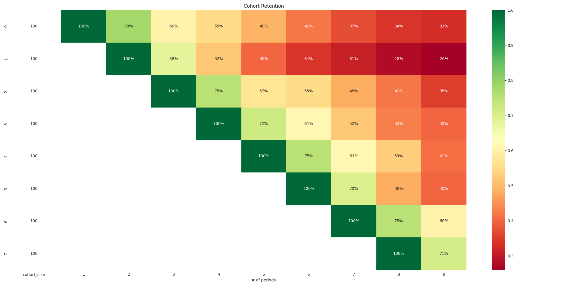

Posterior distributions vs true values

Plot the posterior distributions vs true values

fig, (ax1, ax2, ax3) = plt.subplots(3, figsize=(12, 12))
az.plot_posterior(inference_data, var_names=("alpha",),
                  ref_val=true_alpha,
                  ax=ax1)
az.plot_posterior(inference_data, var_names=("beta",),
                  ref_val=true_beta,
                  ax=ax2)
az.plot_posterior(inference_data, var_names=("conversion_rate",),
                  ref_val=1/true_conversion_rate,
                  ax=ax3)
fig.suptitle(f'True v Recovered values')